Foundations of AI 12. Making Simple Decisions under Uncertainty - PowerPoint PPT Presentation
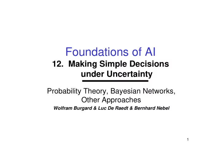
Foundations of AI 12. Making Simple Decisions under Uncertainty Probability Theory, Bayesian Networks, Other Approaches Wolfram Burgard & Luc De Raedt & Bernhard Nebel 1 Contents Motivation Foundations of Probability Theory
Foundations of AI 12. Making Simple Decisions under Uncertainty Probability Theory, Bayesian Networks, Other Approaches Wolfram Burgard & Luc De Raedt & Bernhard Nebel 1
Contents • Motivation • Foundations of Probability Theory • Probabilistic Inference • Bayesian Networks • Alternative Approaches 2
Motivation • In many cases, our knowledge of the world is incomplete (not enough information) or uncertain (sensors are unreliable). • Often, rules about the domain are incomplete or even incorrect – in the qualification problem , for example, what are the preconditions for an action? • We have to act in spite of this! → Drawing conclusions under uncertainty 3
Example • Goal : Be in Freiburg at 9:15 to give a lecture. • There are several plans that achieve the goal: – P 1 : Get up at 7:00, take the bus at 8:15, the train at 8:30, arrive at 9:00 … – P 2 : Get up at 6:00, take the bus at 7:15, the train at 7:30, arrive at 8:00 … – … • All these plans are correct, but → They imply different costs and different probabilities of actually achieving the goal. → P 2 would be the plan of choice, since giving a lecture is very important, and the success rate of P 1 is only 90 - 9 5%. 4
Uncertainty in Logical Rules (1) Example: Expert dental diagnosis system. ∀ p [Symptom(p, toothache) � Disease(p, cavity)] → This rule is incorrect ! Better: ∀ p [Symptom(p, toothache) � Disease(p, cavity) � Disease(p, gum_disease) � …] … but we don’t know all the causes. Perhaps a causal rule is better? ∀ p [Disease(p, cavity) � Symptom(p, toothache)] → Does not allow to reason from symptoms to causes 5 & is still wrong!
Uncertainty in Rules (2) • We cannot enumerate all possible causes, and even if we could … • We don’t know how correct the rules are (in medicine) • … and even if we did, there will always be uncertainty about the patient (the coincidence of having a toothache and a cavity that are unrelated, or the fact that not all tests have been run) → Without perfect knowledge, logical rules do not help much! 6
Uncertainty in Facts Let us suppose we wanted to support the localization of a robot with (constant) landmarks. With the availability of landmarks, we can narrow down on the area. Problem: Sensors can be imprecise. → From the fact that a landmark was perceived, we cannot conclude with certainty that the robot is at that location. → The same is true when no landmark is perceived. → Only the probability increases or decreases. 7
Degree of belief and Probability Theory (1) • We (and other agents) are convinced by facts and rules only up to a certain degree. • One possibility for expressing the degree of belief is to use probabilities . • The agent is 90% (or 0.9) convinced by its sensor information = in 9 out of 10 cases, the information is correct (the agent believes). • Probabilities sum up the “uncertainty” that stems from lack of knowledge. • Probabilities are not to be confused with vagueness. The predicate tall is vague ; the statement, “A man is 1.75–1.80m” tall is uncertain . 8
Uncertainty and Rational Decisions • We have a choice of actions (or plans) • These can lead to different solutions with different probabilities . • The actions have different (subjective) costs • The results have different (subjective) utilities • It would be rational to choose the action with the maximum expected total utility ! → Decision Theory = Utility Theory + Probability Theory 9
Decision-Theoretic Agent Decision Theory : An agent is rational exactly when it chooses the action with the maximum expected utility taken over all results of actions . 10
Unconditional Probabilities (1) P(A) denotes the unconditional probability or prior probability that A will appear in the absence of any other information , for example: P(Cavity) = 0.1 Cavity is a proposition. We obtain prior probabilities from statistical analysis or general rules. 11
Unconditional Probabilities (2) In general, a random variable can take on true and false values, as well as other values: P(Weather=Sunny) = 0.7 P(Weather=Rain) = 0.2 P(Weather=Cloudy) = 0.08 P(Weather=Snow) = 0.02 P(Headache=TRUE) = 0.1 • Propositions can contain equations over random variables. • Logical connectors can be used to build propositions, e.g. P(Cavity � ¬ Insured) = 0.06. 12
Unconditional Probabilities (3) P (x) is the vector of probabilities for the (ordered) domain of the random variable X: P (Headache) = � 0.1, 0.9 � P (Weather) = � 0.7, 0.2, 0.08, 0.02 � define the probability distribution for the random variables Headache and Weather. P (Headache, Weather) is a 4x2 table of probabilities of all combinations of the values of a set of random variables. Headache = TRUE Headache = FALSE Weather = Sunny P(W = Sunny � Headache) P(W = Sunny � ¬ Headache) Weather = Rain Weather = Cloudy Weather = Snow 13
Conditional Probabilities (1) New information can change the probability. Example: The probability of a cavity increases if we know the patient has a toothache. If additional information is available, we can no longer use the prior probabilities! P(A|B) is the conditional or posterior probability of A given that all we know is B: P(Cavity | Toothache) = 0.8 P (X|Y) is the table of all conditional probabilities over all values of X and Y. 14
Conditional Probabilities (2) P (Weather | Headache) is a 4x2 table of conditional probabilities of all combinations of the values of a set of random variables. Headache = TRUE Headache = FALSE Weather = Sunny P(W = Sunny | Headache) P(W = Sunny | ¬ Headache) Weather = Rain Weather = Cloudy Weather = Snow Conditional probabilities result from unconditional probabilities (if P(B)>0) ( per definition ) P(A � B) P(A|B) = P(B) 15
Conditional Probabilities (3) P (X,Y) = P (X|Y) P (Y) corresponds to an equality system: P(W = Sunny � Headache) = P(W = Sunny | Headache) P(Headache) P(W = Rain � Headache) = P(W = Rain | Headache) P(Headache) = � � P(W = Snow � ¬ Headache) = P(W = Snow | ¬ Headache) P( ¬ Headache) 16
Conditional Probabilities (4) P(A � B) P(A|B) = P(B) • Product rule: P(A � B) = P(A|B) P(B) • Analog: P(A � B) = P(B|A) P(A) • A and B are independent if P(A|B) = P(A) (equiv. P(B|A) = P(B)). Then (and only then) it holds that P(A � B) = P(A) P(B). 17
Axiomatic Probability Theory A function P of formulae from propositional logic in the set [0,1] is a probability measure if for all propositions A, B: 1. 0 ≤ P(A) ≤ 1 2. P( true ) = 1 3. P( false ) = 0 4. P(A � B) = P(A) + P(B) – P(A � B) All other properties can be derived from these axioms, for example: P( ¬ A) = 1 – P(A) follows from P(A � ¬ A) = 1 and P(A � ¬ A) = 0. 18
Why are the Axioms Reasonable? • If P represents an objectively observable probability, the axioms clearly make sense. • But why should an agent respect these axioms when it models its own degree of belief? → Objective vs. subjective probabilities The axioms limit the set of beliefs that an agent can maintain. One of the most convincing arguments for why subjective beliefs should respect the axioms was put forward by de Finetti in 1931. It is based on the connection between actions and degree of belief. → If the beliefs are contradictory, then the agent will fail in its environment in the long run! 19
Joint Probability The agent assigns probabilities to every proposition in the domain. An atomic event is an assignment of values to all random variables X 1 , …, X n (= complete specification of a state). Example: Let X and Y be boolean variables. Then we have the following 4 atomic events: X � Y, X � ¬ Y, ¬ X � Y, ¬ X � ¬ Y. The joint probability distribution P (X 1 , …, X n ) assigns a probability to every atomic event . Toothache ¬ Toothache Cavity 0.04 0.06 ¬ Cavity 0.01 0.89 Since all atomic events are disjoint, the sum of all fields is 1 (disjunction of events). The conjunction is necessarily false. 20
Working with Joint Probability All relevant probabilities can be computed using the joint probability by expressing them as a disjunction of atomic events. Examples: P(Cavity � Toothache) = P(Cavity � Toothache) + P( ¬ Cavity � Toothache) + P(Cavity � ¬ Toothache) We obtain unconditional probabilities by adding across a row or column: P(Cavity) = P(Cavity � Toothache) + P(Cavity � ¬ Toothache) P(Cavity � Toothache) 0.04 P(Cavity |Toothache) = = = 0.80 P(Toothache) 0.04+0.01 21
Problems with Joint Probabilities We can easily obtain all probabilities from the joint probability. The joint probability, however, involves k n values, if there are n random variables with k values. → Difficult to represent → Difficult to assess Questions: 1. Is there a more compact way of representing joint probabilities? 2. Is there an efficient method to work with this representation? Not in general, but it can work in many cases. Modern systems work directly with conditional probabilities and make assumptions on the independence of variables in order to simplify calculations. 22
Recommend
More recommend
Explore More Topics
Stay informed with curated content and fresh updates.
