Forecasting and Now-Casting with Disparate Predictors: Dynamic - PowerPoint PPT Presentation

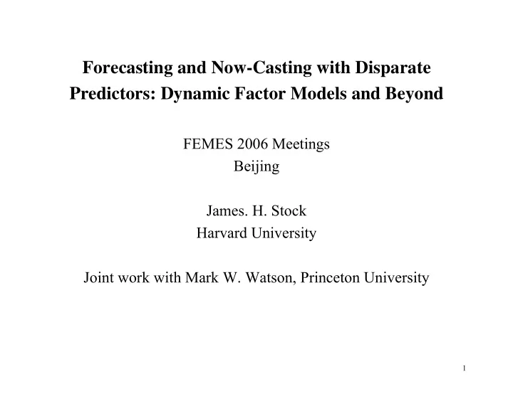
Forecasting and Now-Casting with Disparate Predictors: Dynamic Factor Models and Beyond FEMES 2006 Meetings Beijing James. H. Stock Harvard University Joint work with Mark W. Watson, Princeton University 1

Introduction • The history of macroeconomic forecasting has been an uneasy coexistence of “structural” models and “time series” models. • This talk focuses on a class of models that can incorporate economic theory (as much or as little as desired) into a time series structure – dynamic factor models, using a large number of series. • The data and economic forecasting environment: o there are many predictors (“large n ”) o variables are measured with error (possibly large) o the available time series might be short, might have different start dates and might have different sampling frequencies (mixed monthly-quarterly) o there might be breaks in the individual series, e.g. changes in definitions, collection methods, etc. 2

In this talk I will: • Summarize an exciting modeling framework that has received a lot of recent attention: the dynamic factor model (DFM) o One main message is that, in the DFM, having many time series is a “blessing” of dimensionality, not a “curse” – having many series can make up for deficiencies in any one series. (This will be made more precise.) • Discuss main theoretical results for DFMs • Go through an empirical example for U.S. data with n = 132 variables • Provide a general framework for optimal linear forecasting in a stationary environment and compare the DFM forecasts to the “optimal” (in a specific sense) forecasts – do forecasts based on a small number of factors omit potentially useful information? 3

Outline 1. Introduction 2. Background – VARs and their limitations 3. Dynamic factor models: some theory, VARs v. DFMs, and a survey of recent theoretical results 4. An empirical DFM – US data, 132 series 5. Econometric theory of forecasting using many predictors 6. Empirical forecast evaluation of DFMs vs. other many- predictor methods – US data 4

References *Stock, J.H. and M.W. Watson (2006), “Forecasting with Many Predictors,” Handbook of Economic Forecasting , ch. 10 Stock, J.H. and M.W. Watson (2006), “Implications of Dynamic Factor Models for VAR Analysis,” manuscript, Harvard University Stock, J.H. and M.W. Watson (2006), “An Empirical Comparison of Methods for Forecasting with Many Predictors,” manuscript, Harvard University 5

2. VARs and their Limitations Vector Autoregression (VAR) (Sims, 1980): x 1 t = A 11 (L) x 1 t –1 + A 12 (L) x 2 t –1 + u 1 t x 2 t = A 21 (L) x 1 t –1 + A 22 (L) x 2 t –1 + u 2 t or X t = A(L) X t –1 + u t In general, X t is n × 1 and the VAR has n -variables with p lags of each variable in each equation Drawbacks of VARS • pn 2 parameters – so n cannot be large (6, 9,…) • Can address dimensionality problem using priors, but most priors are ad-hoc (statistical, not economic) • mediocre forecasting performance: too many parameters, sensitive to mis-specification in one of the equations 6

3. Dynamic Factor Models Introduced by Geweke (1975, 1977) (a) Key DFM ideas: • A handful of structural shocks cause the comovements among macro variables at all leads/lags. • That is, the economy follows a dynamic factor model • The “handful” of shocks might be as few as 2! Sargent and Sims (1977), Sargent (1989), Quah and Sargent (1992), Stock and Watson (1989, 1999, 2002b), Giannone, Reichlin, and Sala (2004),… • Recent work on DFMs has focused on large n is a blessing: Stock and Watson (1999, 2002), Ding and Hwang (2001), Forni, Lippi, Hallin, Reichlin (2001), Bai and Ng (2002, 2004, 2006), Bai (2003),… 7

(b) The dynamic factor model X it = λ i (L) f t + u it , i = 1,…, n , Γ (L) f t = η t , X it = t th observation on i th observable variable f t = unobserved factors, q × 1 ( q dynamic factors) λ i (L) f t = “common component” λ i (L) = lag polynomial (“dynamic factor loadings”) u it = idiosyncratic disturbance (possibly serially correlated) cov( f t , u is ) = 0 for all i , s 8

(c) The exact DFM : Eu it u jt = 0, i ≠ j (idiosyncratic disturbances uncorrelated) (d) Spectral factorization : S XX ( ω ) = λ ( e i ω ) S ff ( ω ) λ ( e – i ω ) ′ + S uu ( ω ), where S uu ( ω ) is diagonal under the exact DFM. (e) Estimation when n is small X it = λ i (L) f t + u it , i = 1,…, n , Γ (L) f t = η t , This is a linear state space model, so it can be estimated in the time domain by Gaussian MLE using the Kalman filter to compute the likelihood (Sargent (1989), Stock and Watson (1989)) 9

(f) Forecasting equation for one variable, y t : • Denote one of the X ’s as y t (a variable of special interest) • Suppose u yt follows an autoregression; then y t = λ y (L) f t + u yt , u yt = γ (L) u yt –1 + ε t , ε t serially uncorrelated Then E [ y t +1 | X t , y t , f t , X t –1 , y t –1 , f t –1 ,…] = β (L) f t + γ (L) y t so Y t +1 = β (L) f t + γ (L) Y t + ε t +1 No other X ’s are needed if the f ’s are known – optimal forecasts can be made using only lagged f ’s and lagged Y 10

(g) The approximate DFM • Recall that the exact DFM assumes that all the idiosyncratic disturbances are uncorrelated: Eu it u jt = 0, i ≠ j • The approximate DFM relaxes this assumption Chamberlain-Rothschild (1983), Stock and Watson (1999, 2002a,b), Forni, Hallin, Lippi, Reichlin (2000, 2003a,b, 2004) • The general idea is to bound the eigenvalues of S uu ( ω ) – the correlations among the u ’s cannot be “too large” o e.g. Stock and Watson (2002a): n n ∑∑ − ) < ∞ . 1 | ( | lim n →∞ n E u u it jt = = 1 1 i j 11

(h) Estimation of the factors by principal components When n is large, the factors can be estimated by principal components. The starting point is the static form of the DFM. Suppose λ (L) has degree p and let F t = [ f t ′ … f t – p +1 ′ ] ′ : X it = λ i (L) f t + u it Dynamic form: f t = Γ (L) f t –1 + η t X it = Λ i F t + u i t Static form: (1) F t = Φ (L) F t –1 + G η t (2) where G is r × q ; r = dim( F t ) = number of static factors. 12

DFM estimation by principal components analysis, ctd. X t = Λ F t + u i t ( X t is n × 1, Λ is n × r ) Static form: (1) By analogy to regression, estimate Λ and { F t } by NLLS, T ∑ − − Λ − Λ 1 min ( )'( ) T X F X F Λ ,..., , F F t t t t 1 T = 1 t subject to Λ ′ Λ = I r (identification). Concentrate out { F t }: ′ ∑ − T ′ − − Λ Λ Λ Λ 1 1 min Λ [ ( ) ] T X I X = t t 1 t ′ ∑ ⇔ max Λ tr{( Λ ′ Λ ) –1/2 ′ Λ ′ ˆ Λ ( Λ ′ Λ ) –1/2 where ˆ Σ Σ − T 1 = T X X XX XX = t t 1 t ˆ ⇔ max Λ Λ ′ Σ Λ s.t. Λ ′ Λ = I r , XX ˆ ˆ Λ Σ ⇒ = first r eigenvectors of XX ˆ ˆ ′ Λ ⇒ = = first r principal components of X t . F X t t 13

Distribution Theory for PCA as factor estimator • Connor and Korajczyk (1986) (consistency; exact static FM, T fixed, n → ∞ ) • Stock and Watson (2002a) (consistency; approximate DFM, n , T →∞ , no n / T rate restrictions) • Bai (2003) (asymptotic normality of PCA estimator of the common component at rate min( n 1/2 , T 1/2 ); exact DFM,) • Bai and Ng (2004) (extend Bai (2003) to approximate DFM) • Bai and Ng (2006) (confidence intervals when estimated factors in subsequent regressions) 14

(i) Extension: weighted principal components . Infeasible WLS: T ∑ − − Λ Σ − Λ 1 min ( )' ( ) . X F X F Λ ,..., , F F t t uu t t 1 T = 1 t ˆ ˆ − − Λ Σ Σ Σ 1/2 1/2 ′ Solution: = first q eigenvectors of uu XX uu Feasible weighted PCA : (a) Forni et. al. (2004): ˆ Σ = ˆ – ˆ Σ Σ , uu XX cc ˆ Σ where is estimate of covariance matrix of the common cc component in the DFM, estimated by dynamic PCA (Forni et. al. (2003b) (b) Bovin and Ng (2005): ˆ diag = diag( ˆ Σ Σ ) uu uu (this accords with exact DFM restrictions) 15

(k) Estimation of the number of factors • Number of static factors ( r ): o Bai and Ng (2002) (information criterion applied to eigenvalues of X ′ X , approximate DFM) o Onatski (2005) – formal test for number of static factors based on eigenvalues of X ′ X for number of nonzero eigenvalues (number of principal components to include) • Number of dynamic factors ( q ): o Giannoni, D., L. Reichlin and L. Sala (2004) – heuristic methods based on inspection of eigenvalues of residuals of VAR for F t (static factors) o Amengual and Watson (2006) – extend Bai-Ng to estimate the number of dynamic factors ( q ) by applying information criterion to covariance matrix of residuals from VAR for F t 16

4. An Empirical DFM with U.S. Data The data • n = 132, postwar monthly US o real activity o prices o interest rates and spreads o exchange rates o stock returns o misc • All transformed to “stationarity” by first differencing, logs, etc Base specification VAR(2) for F t , 6 lags for δ (L) 17