For Information on SNAKEs Not in Forsyth and Ponce. Back to - PDF document
Active Contours (SNAKES) For Information on SNAKEs Not in Forsyth and Ponce. Back to boundary detection See Text by Trucco and Verri , or Shapiro and This time using perceptual grouping. Stockman. Kass , Witkin and Terzopoulos ,
Active Contours (SNAKES) For Information on SNAKEs • Not in Forsyth and Ponce. • Back to boundary detection • See Text by Trucco and Verri , or Shapiro and – This time using perceptual grouping. Stockman. • Kass , Witkin and Terzopoulos , IJCV. • This is non - parametric • “Dynamic Programming for Detecting, Tracking, and – We’re not looking for a contour of a specific Matching Deformable Contours”, by Geiger, Gupta, shape. Costa, and Vlontzos , IEEE Trans. PAMI 17(3)294 - 302, 1995 – Just a good contour. • E. N. Mortensen and W. A. Barrett, Intelligent Scissors for Image Composition , in ACM Computer Graphics (SIGGRAPH `95), pp. 191 - 198, 1995 Sometimes edge detectors find the boundary pretty well. Sometimes it’s not enough. Improve Boundary Detection • Integrate information over distance. • Use Gestalt cues – Smoothness – Closure • Get User to Help. Humans integrate contour information. 1
We’ll do something easier than Strategy of Class finding the whole boundary. Finding the best path between two boundary points. • What is a good path? • Given endpoints, how do we find a good path? • What if we don’t know the end points? Note that like all vision this is modeling and optimization . Discrete Grid How do we decide how • Contour should be near edge. good a path • Strength of gradient. is? Which of two paths is • Contour should be smooth better? (good continuation). • Low curvature • Low change of direction of gradient. Review Gradient Smoothness • Discrete Curvature: if you go from p(j - 1) Blackboard: See notes on Class 6 also. to p(j) to p(j+1) how much did direction change? – Be careful with discrete distances. • Change of direction of gradient from p(j - 1) to p(j) 2
Combine into a cost function One Example cost function [ ] ∑ = n + + λ − • Path: p(1), p(2), … p(n). d ( p ( j ), p ( j 1 )) * g ( p ( j ) f ( p ( j 1 ), p ( j ) j 1 [ ] ∑ = n + + λ − d ( p ( j ), p ( j 1 )) * g ( p ( j ) f ( p ( j 1 ), p ( j ) ∇ I 1 j 1 = = ρ g ( p ( j )) l j is some constant + ρ ∇ l 2 j max I j Where j j • d(p(j),p(j+1)) is distance between consecutive grid points f is the angle between the gradient at p(j - 1) and p(j). ( ie , 1 or sqrt(2). Or it could more directly measure curvature of the curve. • g(p(j)) measures strength of gradient � λ is some parameter (Loosely based on “Dynamic Programming for Detecting, Tracking, and Matching Deformable Contours”, by Geiger, Gupta, Costa, and • f measures smoothness, curvature. Vlontzos , IEEE Trans. PAMI 17(3)294 - 302, 1995.) So How do we find the best Example Path? Computer Science at last. A Curve is a path through the grid. Cost depends on each step of the path. We want to minimize cost. Dijkstra’s shortest path algorithm Map problem to Graph link cost 4 9 5 1 0 3 3 3 2 • Algorithm 1. init node costs to ∞ , set p = seed point, cost( p ) = 0 2. expand p as follows: for each of p ’s neighbors q that are not expanded – set cost( q ) = min( cost( p ) + c pq , cost( q ) ) Weight represents cost of going from one pixel to another. Next term in sum. (Seitz) 3
Dijkstra’s shortest path algorithm Dijkstra’s shortest path algorithm 4 9 5 4 9 5 4 9 3 2 4 9 5 5 5 1 1 1 0 3 3 2 1 1 1 0 3 3 3 3 3 3 3 3 2 4 2 3 2 3 3 2 3 • Algorithm • Algorithm 1. init node costs to ∞ , set p = seed point, cost( p ) = 0 1. init node costs to ∞ , set p = seed point, cost( p ) = 0 2. expand p as follows: 2. expand p as follows: for each of p ’s neighbors q that are not expanded for each of p ’s neighbors q that are not expanded – set cost( q ) = min( cost( p ) + c pq , cost( q ) ) – set cost( q ) = min( cost( p ) + c pq , cost( q ) ) » if q ’s cost changed, make q point back to p » if q ’s cost changed, make q point back to p – put q on the ACTIVE list (if not already there) – put q on the ACTIVE list (if not already there) 3. set r = node with minimum cost on the ACTIVE list 4. repeat Step 2 for p = r Dijkstra’s shortest path algorithm Application: Intelligent Scissors 4 3 6 5 3 2 4 9 5 5 3 2 1 1 1 0 3 3 3 3 3 3 4 2 4 3 2 2 3 • Algorithm 1. init node costs to ∞ , set p = seed point, cost( p ) = 0 2. expand p as follows: for each of p ’s neighbors q that are not expanded – set cost( q ) = min( cost( p ) + c pq , cost( q ) ) » if q ’s cost changed, make q point back to p – put q on the ACTIVE list (if not already there) 3. set r = node with minimum cost on the ACTIVE list 4. repeat Step 2 for p = r Results Continuous versions • Can express cost ∇ I ( t ) function as continuous. κ ∫ ( t ) dt • Use continuous ∇ optimization like max I ( s ) gradient descent. • Level Set methods. • These lead to local optima near a starting point. (Seitz Class) demo 4
Why do we need user help? Lessons • Why not run all points shortest path and • Perceptual organization, middle level find best closed curve? knowledge, needed for boundary detection. • Fully automatic methods not good enough yet. • Formulate desired solution then optimize it. 5
This document was created with Win2PDF available at http://www.daneprairie.com. The unregistered version of Win2PDF is for evaluation or non-commercial use only.
Recommend
More recommend
Explore More Topics
Stay informed with curated content and fresh updates.
