Feynman-Kac particle models Coalescent tree based functional - PowerPoint PPT Presentation
Symposium, Univ. Bonn MDV Sept. 2006 Stochastic Algorithms and Markov Processes Feynman-Kac particle models Coalescent tree based functional representations P. DEL MORAL, F. PATRAS, S. RUBENTHALER Lab. J.A. Dieudonn e, Univ. Nice Sophia
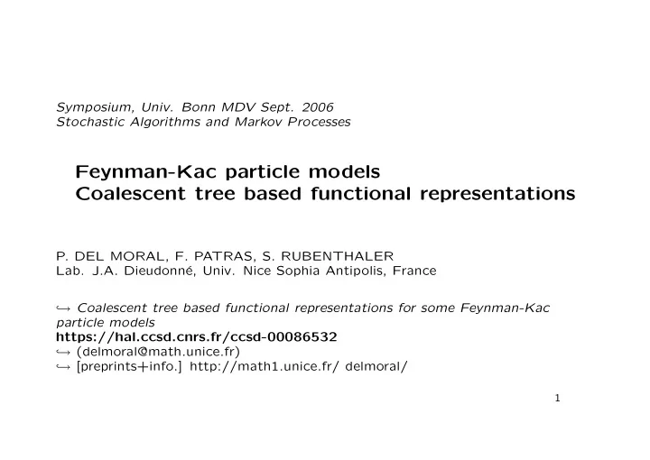
Symposium, Univ. Bonn MDV Sept. 2006 Stochastic Algorithms and Markov Processes Feynman-Kac particle models Coalescent tree based functional representations P. DEL MORAL, F. PATRAS, S. RUBENTHALER Lab. J.A. Dieudonn´ e, Univ. Nice Sophia Antipolis, France → Coalescent tree based functional representations for some Feynman-Kac ֒ particle models https://hal.ccsd.cnrs.fr/ccsd-00086532 ֒ → (delmoral@math.unice.fr) ֒ → [preprints+info.] http://math1.unice.fr/ delmoral/ 1
Introduction • Evolutionary models and Feynman-Kac formulae • Genetic genealogical models and Feynman-Kac limiting measures • Functional representations ≃ precise propagations of chaos expansions . – Combinatorial differential calculus – Permutation group analysis of (colored) forests (wreath product of permutation groups, Hilbert series techniques,. . . ) • (Applications). Discrete time models � Continuous time version = Moran type genetic models ( ∼ joint works with L. Miclo, see also [PhD ⊕ articles] M. Rousset) 2
Evolutionary type models Simple Genetic Branching Algo. Mutation Selection/Branching Metropolis-Hastings Algo. Proposal Acceptance/Rejection Sequential Monte Carlo methods Sampling Resampling (SIR) Filtering/Smoothing Prediction Updating/Correction Particle ∈ Absorbing Medium Evolution Killing/Creation/Anhiling Other Botanical Names: multi-level splitting (Khan-Harris 51), prune enrichment (Rosenbluth 1955), switching algo. (Magill 65), matrix reconfiguration (Hetherington 84), restart (Villen-Altamirano 91), particle filters (Rigal-Salut-DM 92), SIR filters (Gordon-Salmon-Smith 93, Kitagawa 96), go- with-the-winner (Vazirani-Aldous 94), ensemble Kalman-filters (Evensen 1994), quantum Monte Carlo methods (Melik-Nightingale 1999), sequential Monte Carlo Methods (Arnaud Doucet 2001), spawning filters (Fisher-Maybeck 2002), SIR Pilot Exploration Resampling (Liu-Zhang 2002),... 3
⇐ ⇒ Particle Interpretations of Feynman-Kac models Since R. Feynman’s phD. on path integrals 1942 Physics ← → Biology ← → Engineering Sciences ← → Probability/Statistics • Physics : – FKS ∈ nonlinear integro-diff. ´ eq. ( ∼ generalized Boltzmann models). – Spectral analysis of Schr¨ odinger operators and large matrices with nonnegative entries. (particle evolutions in disordered/absorbing media) – Multiplicative Dirichlet problems with boundary conditions. – Microscopic and macroscopic interacting particle interpretations. • Biology : – Self-avoiding walks, macromolecular polymerizations. – Branching and genetic population models. – Coalescent and Genealogical evolutions. 4
• Rare events analysis : – Multisplitting and branching particle models (Restart). – Importance sampling and twisted probability measures. – Genealogical tree based simulation methods. • Advanced Signal processing : – Optimal filtering/smoothing/regulation, open loop optimal control. – Interacting Kalman-Bucy filters. – Stochastic and adaptative grid approximation-models • Statistics/Probability : – Restricted Markov chains (w.r.t terminal values, visiting regions,...) – Analysis of Boltzmann-Gibbs type distributions (simulation, partition functions,...). – Random search evolutionary algorithms, interacting Metropolis/simulated annealing algo.
Simple Genetic evolution/simulation models − → only 2 ingredients!! (Discrete time parameter n ∈ N = { 0 , 1 , 2 , ... } , state spaces E n ( ∈ { Z d , R d , R d × . . . × R d , ... } ) � �� � ( n +1) − times • Mutation/exploration/prediction/proposal : → Markov transitions M n ( x n − 1 , dx n ) from E n − 1 into E n . • Selection/absorption/updating/acceptance : → Potential functions G n from E n into [0 , 1]. 5
A Genetic Evolution Model ⇒ Markov chain ξ n = ( ξ 1 n , . . . , ξ N n ) ∈ E N n = E n × . . . × E n � �� � N − times selection mutation → � ξ n ∈ E N ξ n ∈ E N → ξ n +1 ∈ E N − − − − − − − − − − − − − − − − − − − − − − − − − − − − − − n n n +1 • Selection transition ( ∃ � = types → Ex.: accept/reject) n � � ξ i ξ i n = ξ i G n ( ξ i with proba. n ) [Acceptance] n Otherwise we select a better fitted individual in the current configuration N � ξ i � n = ξ j G n ( ξ j G n ( ξ k with proba. n ) / n ) [Rejection + Selection] n k =1 • Mutation transition n , . ) � n +1 ∼ M n +1 ( � ξ i n � ξ i ξ i 6
A Genealogical tree model Important observation [Historical process] X ′ n ∈ E ′ Markov chain n ⇓ X n = ( X ′ 0 , . . . , X ′ n ) ∈ E n = ( E ′ 0 × . . . × E ′ n ) Markov chain ∈ path spaces → Markov transitions M n ( x n − 1 , dx n ) [elementary extensions] X n +1 = (( X ′ 0 , . . . , X ′ n ) , X ′ n +1 ) = ( X n , X ′ n +1 ) 7
Genetic Evolution Model on Path Spaces=Genealogical tree model X n = ( X ′ 0 , . . . , X ′ G n ( X n ) = G ′ n ( X ′ n ) M n n ) Markov transitions and ↓ Genetic path-valued particle Model � ξ i ( ξ i 0 ,n , ξ i 1 ,n , . . . , ξ i = n,n ) n � ( � 0 ,n , � 1 ,n , . . . , � ξ i ξ i ξ i ξ i n,n ) ∈ E n = ( E ′ 0 × . . . × E ′ = n ) n • Path acceptance/(rejection+selection). • Path mutation = path elementary extensions. 8
Occupation/Empirical measures ( ∀ f n test function on E n ) N N � � n ( f n ) = 1 n ) = 1 η N f n ( ξ i f n ( ξ i 0 ,n , ξ i 1 ,n , . . . , ξ i n,n ) � �� � N N i =1 i =1 i -th ancestral lines ↓ Unbias-particle measures & Unnormalized Feynman-Kac measures : � � γ N η N η N n ( f n ) = n ( f n ) × p ( G p ) − → N →∞ γ n ( f n ) = E ( f n ( X n ) G p ( X p )) 0 ≤ p<n 0 ≤ p<n Notes: n (1) = � → N →∞ γ n (1) = E ( � • f n = 1 ⇒ γ N 0 ≤ p<n η N p ( G p ) − 0 ≤ p<n G p ( X p )) • Path-space models � [ X n = ( X ′ 0 , . . . , X ′ n ) and G n ( X n ) = G ′ n ( X ′ n ) ] ⇒ γ n ( f n ) = E ( f n ( X ′ 0 , . . . , X ′ G ′ p ( X ′ n ) p )) 0 ≤ p<n 9
= ⇒ Occupation measure & Normalized Feynman-Kac measures: N � 1 η N f n ( ξ i n ) = γ N n ( f n ) /γ N n ( f n ) = n (1) − → N →∞ η n ( f n ) = γ n ( f n ) /γ n (1) N i =1 Path-space models [ X n = ( X ′ 0 , . . . , X ′ n ) and G n ( X n ) = G ′ n ( X ′ n ) ] ⇓ n ) � E ( f n ( X ′ 0 , . . . , X ′ 0 ≤ p<n G ′ p ( X ′ p )) E ( � η n ( f n ) = 0 ≤ p<n G ′ p ( X ′ p )) Note: � � − γ N n ( f n ) = η N η N γ n ( f n ) = η n ( f n ) × η p ( G p ) ( ← n ( f n ) × p ( G p )) 0 ≤ p<n 0 ≤ p<n
Motivating example → filtering/hidden Markov chains/Bayesian Stat. Signal process X n = Markov chain ∈ E n Observation/Sensor eq. Y n = H n ( X n , V n ) ∈ F n with P ( H n ( x n , V n ) ∈ dy n ) = g n ( x n , y n ) λ n ( dy n ) Example: Y n = h n ( X n ) + V n ∈ F n = R , with Gaussian noise V n = N (0 , 1) ⇓ P ( h n ( x n ) + V n ∈ dy n ) = (2 π ) − 1 / 2 e − 1 2 ( y n − h n ( x n )) 2 dy n = exp [ h n ( x n ) y n − h 2 N (0 , 1)( dy n ) n ( x n ) / 2] � �� � � �� � λ n ( dy n ) g n ( x n ,y n ) Prediction/filtering/smoothing → Feynman-Kac representation G n ( x n ) = g n ( x n , y n ) η n = Law( X n | Y 0 = y 0 , . . . , Y n − 1 = y n − 1 ) = Law( X ′ 0 , . . . , X ′ n | Y 0 = y 0 , . . . , Y n − 1 = y n − 1 ) 10
Rather complete asymptotic theory ( n, N ) → ∞ (usual LLN, CLT, LDP,...) → F-K Formulae, Genealogical and IPS , Springer (2004) + References therein ֒ Some examples: • Weak convergence [ p ≥ 1 + F n not too large + regular mutations] (JTP 2000, joint work with M. Ledoux) √ n ( f n ) − η n ( f n ) | p ) 1 /p ≤ c ( p ) / | η N sup E ( sup N n ≥ 0 f n ∈F n √ n (1 ] −∞ ,x ] ) − η n (1 ] −∞ ,x ] ) | p ) 1 /p ≤ c ( p ) / | η N Ex : E n = R , F n = { 1 ] −∞ ,x ] ; x ∈ R } ⇒ sup E (sup N n ≥ 0 x ∈ R • Propagation-of-chaos estimates [ q ≤ N finite block size] (TVP+SIAM PTA 2006, joint work with A. Doucet) + 1 P N n,q := Law( ξ 1 n , . . . , ξ q n ) ≃ η ⊗ q N ∂ 1 P n,q ∂ 1 P n,q � ∂ 1 P n,q � tv ≤ c q 2 with signed meas. s.t. sup n n ≥ 0 11
Problem : Pb : Find a functional representation at any order? + 1 N ∂ 1 P n,q + . . . + 1 1 P N n,q ≃ η ⊗ q N k ∂ k P n,q + N k +1 ∂ k P N n n,q with a bounded remainder measure sup N ≥ 1 � ∂ k +1 P N n,q � tv < ∞ Consequences : • Sharp + strong propagations of chaos estimates at any order. • Wick product formulae on forests. • Sharp L p -mean error bounds. • Law of large numbers for U -statistics for interacting processes. • . . . 12
Tensor product measures � � n ) ⊗ q = 1 1 n ) ⊙ q = ( η N ( η N and δ ξ a δ ξ a � N q n ( N ) q n a ∈ [ N ] [ q ] a ∈� q,N � with ( ξ a (1) , . . . , ξ a ( q ) ξ a := ) n n n N q mappings [ q ] := { 1 , . . . , q } � [ N ] := { 1 , . . . , N } ; [ N ] [ q ] := � q, N � := ( N ) q := N ! / ( N − q )! one-to-one mappings 13
Recommend
More recommend
Explore More Topics
Stay informed with curated content and fresh updates.
