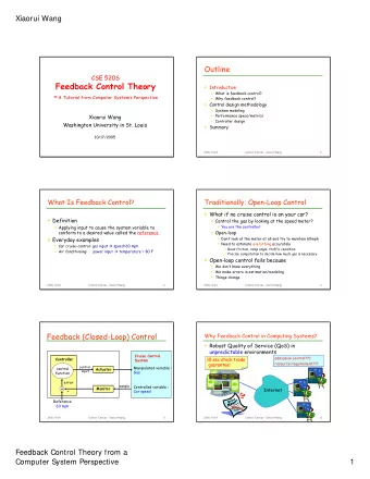
Feedback Control Theory a Computer System s Perspective - PowerPoint PPT Presentation
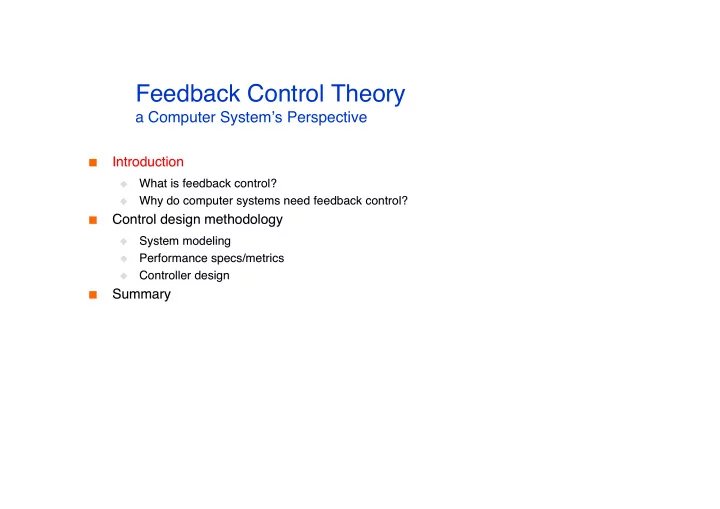
Feedback Control Theory a Computer System s Perspective Introduction Introduction What is feedback control? What is feedback control? Why do computer systems need feedback control? Why do computer systems need feedback
Feedback Control Theory a Computer System ʼ s Perspective Introduction Introduction What is feedback control? What is feedback control? Why do computer systems need feedback control? Why do computer systems need feedback control? Control design methodology Control design methodology System modeling System modeling Performance specs/metrics Performance specs/metrics Controller design Controller design Summary Summary
Control Applying input to cause system variables to conform to desired values called Applying input to cause system variables to conform to desired values called the reference reference. . the speed=60 mph Cruise-control car: f_engine(t)=? Cruise-control car: f_engine(t)=? speed=60 mph T_response=5 sec Resource allocation? E-commerce server: Resource allocation? E-commerce server: T_response=5 sec Delay = 1 sec Flow rate? Embedded networks: Flow rate? Embedded networks: Delay = 1 sec Computer systems: QoS guarantees Computer systems: QoS guarantees
Open-loop control Compute control input without continuous variable measurement Compute control input without continuous variable measurement Simple Simple Need to know EVERYTHING Need to know EVERYTHING ACCURATELY ACCURATELY to work right to work right Cruise-control car: Cruise-control car: friction(t), ramp_angle(t) friction(t), ramp_angle(t) E-commerce server: E-commerce server: Workload (request arrival rate? resource Workload (request arrival rate? resource consumption?); system (service time? fa ilures ?) consumption?); system (service time? fa ilures ?) Open-loop control fails when Open-loop control fails when We don ʼ We don ʼ t know everything t know everything We make errors in estimation/modeling We make errors in estimation/modeling Things change Things change
Feedback (close-loop) Control Controlled System Controller control manipulated control Actuator input variable function error sample controlled + - Monitor variable reference
Feedback (close-loop) Control Measure variables and use it to compute control input Measure variables and use it to compute control input More complicated (so we need control theory) More complicated (so we need control theory) Continuously measure & correct Continuously measure & correct Cruise-control car: Cruise-control car: measure speed & change engine force measure speed & change engine force Ecommerce server: Ecommerce server: measure response time & admission control measure response time & admission control Embedded network: Embedded network: measure collision & change backoff window measure collision & change backoff window Feedback control theory makes it possible to control well even if Feedback control theory makes it possible to control well even if We don ʼ We don ʼ t know everything t know everything We make errors in estimation/modeling We make errors in estimation/modeling Things change Things change
Why feedback control? Open, unpredictable environments Deeply embedded networks: interaction with physical environments Deeply embedded networks: interaction with physical environments Number of working nodes Number of working nodes Number of interesting events Number of interesting events Number of hops Number of hops Connectivity Connectivity Available bandwidth Available bandwidth Congested area Congested area Internet: E-business, on-line stock broker Internet: E-business, on-line stock broker Unpredictable off-the-shelf hardware Unpredictable off-the-shelf hardware
Why feedback control? We want QoS guarantees Deeply embedded networks Deeply embedded networks Update intruder position every 30 sec Update intruder position every 30 sec Report fire <= 1 min Report fire <= 1 min E-business server E-business server Purchase completion time <= 5 sec Purchase completion time <= 5 sec Throughput >= 1000 transaction/sec Throughput >= 1000 transaction/sec The problem: provide QoS guarantees in open, unpredictable The problem: provide QoS guarantees in open, unpredictable environments environments
Advantage of feedback control theory Adaptive resource management heuristics Adaptive resource management heuristics L Laborious design/tuning/testing iterations aborious design/tuning/testing iterations N Not enough confidence in face of untested workload ot enough confidence in face of untested workload Queuing theory Queuing theory Doesn Doesn ʼ ʼ t handle feedbacks t handle feedbacks Not good at characterizing transient behavior in overload Not good at characterizing transient behavior in overload Feedback control theory Feedback control theory Systematic theoretical approach for analysis and design Systematic theoretical approach for analysis and design Predict system response and stability to input Predict system response and stability to input
Outline Introduction Introduction What is feedback control? What is feedback control? Why do today ʼ Why do today ʼ s computer systems need feedback control? s computer systems need feedback control? Control design methodology Control design methodology System modeling System modeling Performance specs/metrics Performance specs/metrics Controller design Controller design Summary Summary
Control design methodology Controller Modeling Design Dynamic model Control algorithm analytical Root-Locus system IDs PI Control Satisfy Requirement Performance Specifications Analysis
System Models Linear Linear vs vs. non-linear (differential . non-linear (differential eqns eqns) ) Deterministic vs vs. Stochastic . Stochastic Deterministic Time-invariant Time-invariant vs vs. Time-varying . Time-varying Are coefficients functions of time? Are coefficients functions of time? Continuous-time vs vs. Discrete-time . Discrete-time Continuous-time System ID vs System ID vs. First Principle . First Principle
Dynamic Model Computer systems are dynamic dynamic Computer systems are Current output depends on “ Current output depends on “history history” ” Characterize relationships among system variables Characterize relationships among system variables Differential equations (time domain) Differential equations (time domain) • • • • • • a y ( t ) a y ( t ) a y ( t ) b u ( t ) b u ( t ) + + = + 2 1 0 1 0 • Transfer functions (frequency domain) Y ( s ) = G ( s ) U ( s ) b s b c c + 1 0 1 2 G ( s ) = = + 2 a s a s a s p s p + + ! ! 2 1 0 1 2 • Block diagram (pictorial) Y(s) C(s) G(s) R(s) -
Example Utilization control in a video server Periodic task T Periodic task T i i corresponding to each video stream i corresponding to each video stream i c[i]: processing time, p[i]: period c[i]: processing time, p[i]: period Stream i Stream i ʼ ʼ s s requested CPU utilization: u[i]=c[i]/p[i] requested CPU utilization: u[i]=c[i]/p[i] Total CPU utilization: U(t)= : U(t)= Σ Σ {k} u[k], {k} is the set of active streams Total CPU utilization {k} u[k], {k} is the set of active streams Completion rate Completion rate: : R R c c (t)= ( (t)= ( Σ Σ { } u[m])/ u[m])/ Δ Δ t t, where {m} is the set of terminated video , where {m} is the set of terminated video {kc kc} streams during [t, t+ streams during [t, t+ Δ Δ t t] ] Unknown Unknown Admission rate: R : R a (t)= ( Σ Σ {ka} u[j])/ Δ t, where {j} is the set of admitted streams during [t, , where {j} is the set of admitted streams during [t, Admission rate a (t)= ( {ka} u[j])/ Δ t t+ t+ Δ Δ t t] ] Problem: design an admission controller to guarantee U(t)= Problem: design an admission controller to guarantee U(t)=U U s s regardless of regardless of R R c c (t) (t)
Model Differential equation • Error: E(t)=U s -U(t) t ! • Model (differential equation): U ( t ) ( R ( ) R ( )) d = # " # # a c 0 # = • Controller C? E(t) ⇒ R a (t) R a (t) - U s C? U(t) CPU R c (t)
A Diversion to Math System representations Three ways of system modeling Three ways of system modeling • Time domain: convolution; differential equations. t ! u(t) y ( t ) g ( t ) * u ( t ) g ( t ) u ( ) d g(t) y(t) = = " # # # 0 • s (frequency) domain: multiplication Y ( s ) G ( s ) U ( s ) U(s) Y(s) G(s) = • Block diagram: pictorial s-domain is a simple & powerful “language” for control analysis
Recommend
More recommend
Explore More Topics
Stay informed with curated content and fresh updates.
