Face Recognition Intro to recognition PCA and Eigenfaces LDA - PowerPoint PPT Presentation
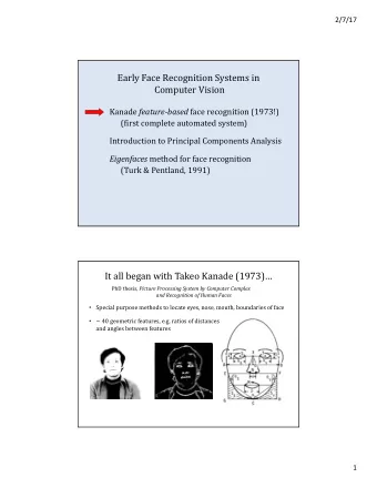
COS 429: COMPUTER VISON Face Recognition Intro to recognition PCA and Eigenfaces LDA and Fisherfaces Face detection: Viola & Jones (Optional) generic object models for faces: the Constellation Model Reading: Turk
COS 429: COMPUTER VISON Face Recognition • Intro to recognition • PCA and Eigenfaces • LDA and Fisherfaces • Face detection: Viola & Jones • (Optional) generic object models for faces: the Constellation Model Reading: Turk & Pentland, ???
Face Recognition • Digital photography
Face Recognition • Digital photography • Surveillance
Face Recognition • Digital photography • Surveillance • Album organization
Face Recognition • Digital photography • Surveillance • Album organization • Person tracking/id.
Face Recognition • Digital photography • Surveillance • Album organization • Person tracking/id. • Emotions and expressions
Face Recognition • Digital photography • Surveillance • Album organization • Person tracking/id. • Emotions and expressions • Security/warfare • Tele-conferencing • Etc.
What’s ‘recognition’? vs. Identification or Discrimination
What’s ‘recognition’? vs. Identification or Categorization or Classification Discrimination
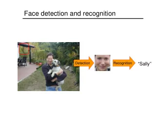
What’s ‘recognition’? Yes, there are faces localization No Identification or Categorization or Classification Discrimination
What’s ‘recognition’? Yes, there is John Lennon localization No Identification or Categorization or Classification Discrimination
What’s ‘recognition’? Detection or Localizatoin John Lennon localization No Identification or Categorization or Classification Discrimination
What’s ‘recognition’? Detection or Localizatoin localization No Identification or Categorization or Classification Discrimination
What’s ‘recognition’? Detection or Localizatoin localization No Identification or Categorization or Classification Discrimination
Today’s agenda Detection or Localizatoin 3. AdaBoost 4. Constellation model localization 1. PCA & Eigenfaces 2. LDA & Fisherfaces No Identification or Categorization or Classification Discrimination
Eigenfaces and Fishfaces • Introduction • Techniques – Principle Component Analysis (PCA) – Linear Discriminant Analysis (LDA) • Experiments
The Space of Faces = + • An image is a point in a high dimensional space – An N x M image is a point in R NM – We can define vectors in this space as we did in the 2D case [Thanks to Chuck Dyer, Steve Seitz, Nishino]
Key Idea χ = P x ˆ { } • Images in the possible set are highly correlated. RL • So, compress them to a low-dimensional subspace that captures key appearance characteristics of the visual DOFs. • EIGENFACES: [Turk and Pentland] USE PCA!
� Two simple but useful techniques For example, a generative graphical model: P(identity,image) = P(identiy|image) P(image) Preprocessing model (can be performed by PCA)
Principal Component Analysis (PCA) Principal Component Analysis (PCA) • PCA is used to determine the most representing features among data points. – It computes the p-dimensional subspace such that the projection of the data points onto the subspace has the largest variance among all p-dimensional subspaces.
Illustration of PCA Illustration of PCA x2 x2 4 4 6 6 1 1 2 2 5 5 3 3 X1’ x1 x1 One projection PCA projection
Illustration of PCA Illustration of PCA 2rd principal component x 2 x 1 1 st principal component
Eigenface for Face Recognition for Face Recognition Eigenface • PCA has been used for face image representation/compression, face recognition and many others. • Compare two faces by projecting the images into the subspace and measuring the EUCLIDEAN distance between them.
Mathematical Formulation Find a transformation, W, m-dimensional Orthonormal n-dimensional Total scatter matrix: W opt corresponds to m eigen- vectors of S T
Eigenfaces • PCA extracts the eigenvectors of A – Gives a set of vectors v 1 , v 2 , v 3 , ... – Each one of these vectors is a direction in face space • what do these look like?
Projecting onto the Eigenfaces • The eigenfaces v 1 , ..., v K span the space of faces – A face is converted to eigenface coordinates by
Algorithm Algorithm Training Training 1. Align training images x 1 , x 2 , …, x N Note that each image is formulated into a long vector! 2. Compute average face u = 1/N Σ x i 3. Compute the difference image φ i = x i – u
Algorithm Algorithm 4. Compute the covariance matrix (total scatter matrix) S T = 1/N Σ φ i φ iT = BB T , B=[ φ 1 , φ 2 … φ N ] 5. Compute the eigenvectors of the covariance matrix , W Testing 1. Projection in Eigenface Projection ω i = W (X – u ), W = {eigenfaces} 2. Compare projections
Illustration of Eigenfaces Eigenfaces Illustration of The visualization of eigenvectors: These are the first 4 eigenvectors from a training set of 400 images (ORL Face Database). They look like faces, hence called Eigenface.
Eigenfaces look somewhat like generic faces.
Eigenvalues Eigenvalues
Reconstruction and Errors Reconstruction and Errors P = 4 P = 200 P = 400 Only selecting the top P eigenfaces � reduces the dimensionality. Fewer eigenfaces result in more information loss, and hence less discrimination between faces.
Summary for PCA and Eigenface Eigenface Summary for PCA and • Non-iterative, globally optimal solution • PCA projection is optimal for reconstruction from a low dimensional basis, but may NOT be optimal for discrimination…
Linear Discriminant Analysis (LDA) Linear Discriminant Analysis (LDA) • Using Linear Discriminant Analysis (LDA) or Fisher’s Linear Discriminant (FLD) • Eigenfaces attempt to maximise the scatter of the training images in face space, while Fisherfaces attempt to maximise the between class scatter , while minimising the within class scatter .
Illustration of the Projection Illustration of the Projection � Using two classes as example: x2 x2 x1 x1 Poor Projection Good Projection
Comparing with PCA Comparing with PCA
Variables { } 1 L • N Sample images: x , , x N { } • c classes: χ χ 1 L , , c 1 μ = ∑ x • Average of each class: i k N ∈ χ x i k i • Total average: 1 N μ = ∑ x k N = k 1
Scatters ( )( ) T = − μ − μ ∑ S x x • Scatter of class i: i k i k i ∈ χ x k i c = • Within class scatter: ∑ S S W i = i 1 c ( )( ) = χ μ − μ μ − μ T ∑ S • Between class scatter: B i i i = i 1 = + • Total scatter: S S S T W B
2 x1 S + Illustration 1 S = S W 2 S x2 1 S B S
Mathematical Formulation (1) y = After projection: T W x k k ~ B = T S W S W Between class scatter (of y’s): B ~ W = T Within class scatter (of y’s): S W S W W
Mathematical Formulation (2) • The desired projection: ~ T W S W S B = B = W arg max arg max ~ opt T S W S W W W W W • How is it found ? � Generalized Eigenvectors = λ = K S w S w i 1 , , m B i i W i Data dimension is much larger than the n >> number of samples N ( ) ≤ − Rank S N c The matrix is singular: S W W
Fisherface (PCA+FLD) N − z = T • Project with PCA to space c W x k pca k = T W W S W arg max pca T W y = T − W z • Project with FLD to space c 1 k fld k T T W W S W W pca B pca = W arg max fld T T W W S W W W pca W pca
Illustration of FisherFace • Fisherface
Results: Eigenface vs. Fisherface (1) • Input: 160 images of 16 people • Train: 159 images • Test: 1 image • Variation in Facial Expression, Eyewear, and Lighting With Without 3 Lighting 5 expressions glasses glasses conditions
Eigenface vs. Fisherface (2)
discussion • Removing the first three principal components results in better performance under variable lighting conditions • The Firsherface methods had error rates lower than the Eigenface method for the small datasets tested.
Today’s agenda Detection or Localizatoin 3. AdaBoost 4. Constellation model localization 1. PCA & Eigenfaces 2. LDA & Fisherfaces No Identification or Categorization or Classification Discrimination
Robust Face Detection Using AdaBoost • Brief intro on (Ada)Boosting • Viola & Jones, 2001 – Weak detectors: Haar wavelets – Integral image – Cascade – Exp. & Res. Reference: P. Viola and M. Jones (2001) Robust Real-time Object Detection, IJCV.
Discriminative methods Object detection and recognition is formulated as a classification problem. The image is partitioned into a set of overlapping windows … and a decision is taken at each window about if it contains a target object or not. Decision boundary Background Where are the screens? Computer screen Bag of image patches In some feature space
Recommend
More recommend
Explore More Topics
Stay informed with curated content and fresh updates.
