11/27/2006 Massachusetts Institute of Technology Context Optimal - PDF document

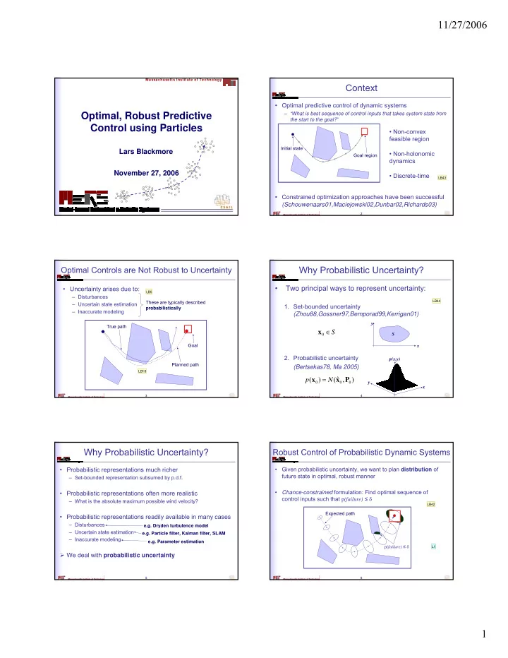
11/27/2006 Massachusetts Institute of Technology Context • Optimal predictive control of dynamic systems – “What is best sequence of control inputs that takes system state from Optimal, Robust Predictive the start to the goal?” Control using Particles • Non-convex feasible region Initial state Lars Blackmore • Non-holonomic Goal region dynamics November 27, 2006 • Discrete-time LB43 • Constrained optimization approaches have been successful (Schouwenaars01,Maciejowski02,Dunbar02,Richards03) 2 Why Probabilistic Uncertainty? Optimal Controls are Not Robust to Uncertainty • Two principal ways to represent uncertainty: • Uncertainty arises due to: LB5 – Disturbances LB44 These are typically described – Uncertain state estimation 1. Set-bounded uncertainty probabilistically – Inaccurate modeling (Zhou88,Gossner97,Bemporad99,Kerrigan01) y True path ∈ x S 0 S Goal x 2. Probabilistic uncertainty p(x,y) Planned path (Bertsekas78, Ma 2005) LB18 = ˆ ( ) ( , ) p x N x P 0 0 0 y x 3 4 Why Probabilistic Uncertainty? Robust Control of Probabilistic Dynamic Systems • Probabilistic representations much richer • Given probabilistic uncertainty, we want to plan distribution of future state in optimal, robust manner – Set-bounded representation subsumed by p.d.f. • Chance-constrained formulation: Find optimal sequence of • Probabilistic representations often more realistic control inputs such that p (failure) ≤ δ – What is the absolute maximum possible wind velocity? LB42 Expected path • Probabilistic representations readily available in many cases – Disturbances e.g. Dryden turbulence model – Uncertain state estimation e.g. Particle filter, Kalman filter, SLAM – Inaccurate modeling e.g. Parameter estimation p (failure) ≤ δ L1 � We deal with probabilistic uncertainty 5 6 1

Slide 2 LB43 Mention: Example: UAV path planning using Mixed Integer Linear Programming Lars Blackmore, 8/18/2006 Slide 3 LB5 Relate to UAV example Lars Blackmore, 8/14/2006 LB18 stress optimal paths particularly bad Lars Blackmore, 8/15/2006 Slide 4 LB44 Spend a little more time on this Lars Blackmore, 8/18/2006 Slide 6 LB42 stress the trade of performance vs conservatism Lars Blackmore, 8/18/2006 L1 mention the 3 challenges Lars, 8/20/2006

11/27/2006 Problem Statement Chance-constrained Control: Prior Work • Prior work developed chance-constrained Model Predictive Control (Li00, VanHessem04) • Design a finite, optimal sequence of control – Restricted to case of Gaussian uncertainty inputs u 0:T-1 such that system state trajectory leaves feasible region with probability at most δ – Restricted to control within convex regions [ ] ( , ) • We extend this work to arbitrary uncertainty • Cost function: h u x ( , ) � E h u x 0 : − 1 1 : T T 0 : − 1 1 : T T distributions and non-convex regions • Feasible region: F LB37 = ν � Chance-constrained particle control ( , , ) • System dynamics: x f u x 0 : − 1 0 0 : − 1 t t t t Random variables with known p.d.f.s Random variable with p.d.f. (at least approximately) to be optimized 7 8 Particles: Probabilistic Properties Chance-constrained Particle Control: Intuition • In estimation, Kalman Filters have been very successful for • Particles can approximate arbitrary distributions: linear systems, Gaussian noise – Draw N samples x (i) from a r.v. X with distribution p(x) – State distribution given model and observations can be calculated – Distribution approximated with delta functions at samples: analytically p(x) 1 N ∑ ≈ δ ( ) ( ) p x x • More recently, Particle Filters have been successful for ( ) i x N = 1 i nonlinear systems, with non-Gaussian noise x Samples drawn from X – State distribution is approximated by a number of particles 1 N ∫ ∑ ∫ ( ∈ ) = ( ) ≈ δ ( ) = fraction of particles in P X S p x dx x dx S – Convergence of approximation to true distribution as number of ( i ) x N S S = i 1 particles tends to infinity • Convergence results: – Number of particles used determined by available resources 1 N ∑ ( ) ⎯ ⎯ almost ⎯ surely ⎯ → → ∞ ( i ) [ ( )] as LB45 f x E f X N N • Idea: Use particles for anytime robust control = 1 i ⎯ almost ⎯ ⎯ surely ⎯ → ∈ → ∞ fraction of particles in set ( ) as S p X S N – Control the distribution of particles to achieve a probabilistic goal LB20 9 10 Technical Approach Technical Approach • Question: How can particles be used to solve chance- 1. Use particles to sample random variables constrained probabilistic control problem? ν p ν ( ) ~ ( ) ( i ) ~ ( ) = Κ = Κ i 1 0 x p x i N t T 0 0 t t • Chance-constrained particle control: 1. Use particles to sample random variables (noise, initial position, Goal Region disturbances) 2. Calculate future state trajectory for each particle leaving explicit dependence on control inputs u 0:T-1 Obstacle 1 3. Express probabilistic optimization problem approximately in terms of particles 4. Solve approximate deterministic optimization problem for u 0:T-1 Initial state distribution Obstacle 2 � Approximate optimization goal tends to true goal as number of Particles approximating particles tends to infinity initial state distribution 11 12 2

Slide 7 LB37 "state depends on x_0 and v which are... because they are random variables, x_t is also." Lars Blackmore, 8/16/2006 Slide 9 LB45 note anytime Lars Blackmore, 8/18/2006 Slide 10 LB20 these are used in filtering --> I will use for control Lars Blackmore, 8/15/2006

11/27/2006 Technical Approach Technical Approach 2. Calculate future state trajectory for each particle leaving 2. Calculate future state trajectory for each particle leaving explicit dependence on control inputs u 0:T-1 explicit dependence on control inputs u 0:T-1 ⎡ ⎤ ⎡ ⎤ ( ) ( ) x i x i 1 1 ⎢ ⎥ ⎢ ⎥ ( ) = ( , ( ) , ν ( ) ) ( ) = ( , ( ) , ν ( ) ) i i i ( ) = Μ i i i ( ) = Μ x f u x i x f u x i x ⎢ ⎥ x ⎢ ⎥ 0 : − 1 0 0 : − 1 1 : 0 : − 1 0 0 : − 1 1 : t t t t T t t t t T ⎢ ⎥ ⎢ ⎥ ( ) ( ) i i ⎣ x ⎦ ⎣ x ⎦ T T Particles 1…N Goal Region Goal Region Particle 1 for u = u B t=4 for u = u B LB38 Obstacle 1 Obstacle 1 t=3 LB24 LB21 t=4 Particles 1…N Particle 1 for u = u A t=2 t=3 for u = u A t=2 Obstacle 2 Obstacle 2 t=1 t=1 t=0 t=0 13 14 Technical Approach Technical Approach 3. Express probabilistic optimization problem approximately 4. Solve approximate deterministic optimization in terms of particles problem for u 0:T-1 δ = 0.1 LB46 Goal Region Goal Region Fraction of particles 10% of particles fail t=4 Sample mean of cost failing approximates in optimal solution t=4 function approximates probability of failure true expectation: Obstacle 1 [ ] Obstacle 1 ( , ) E h u x t=3 − 0 : T 1 1 : T t=3 Sample mean 1 N ∑ ≈ ( ) ( , i ) h u x approximates − 0 : T 1 1 : T t=2 t=2 N state mean = 1 Obstacle 2 i Obstacle 2 t=1 t=1 t=0 t=0 15 16 Convergence Convergence As N � ∞ , approximation becomes exact As N � ∞ , approximation becomes exact – – Goal Region Goal Region 10% probability of failure Obstacle 1 Obstacle 1 Obstacle 2 Obstacle 2 17 18 3

Slide 13 LB21 This is easy to do because all uncertainty has been removed Lars Blackmore, 8/15/2006 Slide 14 LB24 highlight every particle has same control input Lars Blackmore, 8/15/2006 LB38 stress a particle is a _trajectory_ Lars Blackmore, 8/16/2006 Slide 15 LB46 MAX failure rate Lars Blackmore, 8/18/2006