f ( r ) r = a where r is known as the index, a and b are the - PDF document

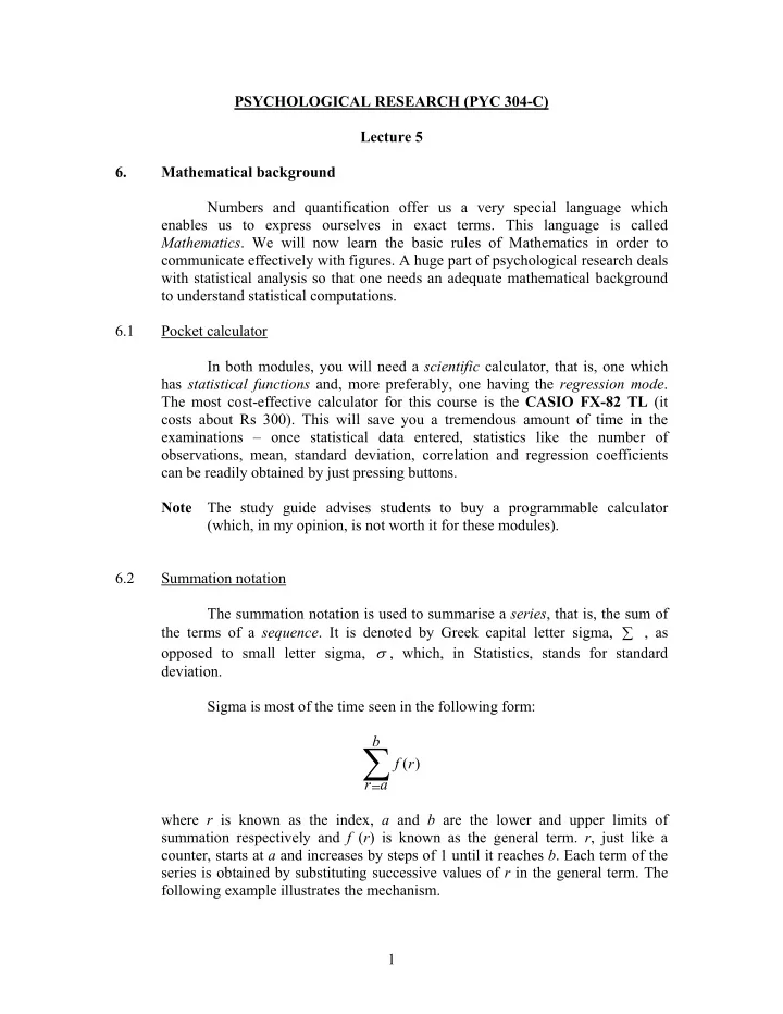
PSYCHOLOGICAL RESEARCH (PYC 304-C) Lecture 5 6. Mathematical background Numbers and quantification offer us a very special language which enables us to express ourselves in exact terms. This language is called Mathematics . We will now learn the basic rules of Mathematics in order to communicate effectively with figures. A huge part of psychological research deals with statistical analysis so that one needs an adequate mathematical background to understand statistical computations. 6.1 Pocket calculator In both modules, you will need a scientific calculator, that is, one which has statistical functions and, more preferably, one having the regression mode . The most cost-effective calculator for this course is the CASIO FX-82 TL (it costs about Rs 300). This will save you a tremendous amount of time in the examinations – once statistical data entered, statistics like the number of observations, mean, standard deviation, correlation and regression coefficients can be readily obtained by just pressing buttons. Note The study guide advises students to buy a programmable calculator (which, in my opinion, is not worth it for these modules). 6.2 Summation notation The summation notation is used to summarise a series , that is, the sum of the terms of a sequence . It is denoted by Greek capital letter sigma, ∑ , as opposed to small letter sigma, σ , which, in Statistics, stands for standard deviation. Sigma is most of the time seen in the following form: b ∑ f ( r ) r = a where r is known as the index, a and b are the lower and upper limits of summation respectively and f ( r ) is known as the general term. r , just like a counter, starts at a and increases by steps of 1 until it reaches b . Each term of the series is obtained by substituting successive values of r in the general term. The following example illustrates the mechanism. 1

6.2.1 Example ∑ 6 [ ] [ ] [ ] + = + + + + + + = + + + + = ( 2 k 1 ) 2 ( 2 ) 1 2 ( 3 ) 1 ... 2 ( 6 ) 1 5 7 9 11 13 45 . = k 2 Here, the index (counter) is k . It can be observed that k takes on an initial value of 2 (the lower limit) and increases by steps of 1 until it reaches the upper limit 6. Every value that k assumes is substituted in the general term (2 k + 1) in order to generate a term of the series. Obviously, the terms are added up since Sigma stands for summation. In Statistics, however, we do not actually evaluate such expressions numerically but rather use the summation notation strictly for summarisation purposes. This is because the upper limit is generally non-numerical, that is, a n variable. We deal mostly with expressions of the form ∑ x . If expanded, this i = i 1 summation cannot be evaluated since it only gives the expression + + + + + x x x ... x x . − 1 1 2 3 n n Such expressions are found in the formulae for arithmetic mean and standard deviation. In this module, students are simply required to recognise the summation notation and understand its meaning so that they can at least use relevant statistical functions on calculators. 7. Presentation of data Once information has been collected, it has to be classified and organised in such a way that it becomes easily readable, that is, converted to data. Before calculation of descriptive statistics, it is sometimes a good idea to present it on charts, diagrams or graphs. Most people find diagrams more helpful than figures in the sense that these present data more meaningfully. In this module, we will only consider the presentation of data in the form of histograms and frequency polygons (read the properties of histograms and frequency polygons in Sections 7.3 and 7.4). 7.1 Ungrouped data This type of information occurs as individual observations, usually as a table or array of disorderly values. These observations are to be firstly arranged in some order (ascending or descending if they are numerical) or simply grouped together in the form of a frequency table before proper presentation on diagrams is possible. 2

The following will be used as an example of ungrouped data throughout section 6.1 of the notes. 7.1.1 Example The following data represent the age of students attending full-time B Sc. courses at De Chazal Du Mée Business School : 22 19 21 22 22 22 19 24 21 22 22 22 21 23 21 21 23 24 22 23 21 21 20 21 21 21 23 22 21 21 22 23 22 22 23 21 22 19 22 22 21 22 21 22 20 21 23 21 22 22 23 21 21 23 22 22 22 23 20 23 21 22 21 22 22 21 21 22 23 21 20 21 22 23 21 21 22 22 23 19 22 21 21 20 22 23 22 22 21 23 22 21 23 21 22 23 20 21 22 22 22 19 21 22 22 22 19 24 21 22 22 22 21 23 21 21 23 24 22 23 21 21 20 21 21 21 23 22 21 21 22 23 22 22 23 21 22 19 22 22 21 22 21 22 20 21 23 21 22 22 23 21 21 23 22 22 22 23 20 19 21 22 21 22 22 21 21 22 23 21 20 21 22 23 21 21 22 22 23 23 22 21 21 20 22 23 22 22 21 23 22 21 23 21 22 23 20 21 22 22 22 19 21 22 22 22 19 24 21 22 22 22 21 23 21 21 23 24 22 23 21 21 20 21 21 21 23 22 21 21 22 23 22 22 23 21 22 19 22 22 21 22 21 22 20 21 23 21 22 22 23 21 21 23 22 22 22 23 21 22 21 22 21 22 22 21 21 22 23 21 20 21 22 23 21 21 22 22 23 21 22 21 21 20 22 23 22 22 21 23 22 21 23 21 22 23 20 21 22 22 22 19 21 22 22 22 19 24 21 22 22 22 21 23 21 21 23 24 22 23 21 21 20 21 21 21 23 22 21 21 22 23 22 22 23 21 22 19 22 22 21 22 21 22 20 21 23 21 22 22 23 21 21 23 22 22 22 23 20 23 21 22 21 22 22 21 21 22 23 21 20 21 22 23 21 21 22 22 23 22 22 21 21 20 22 23 22 22 21 23 22 21 23 21 22 23 20 21 22 Table 7.1.1.1 (The above information has been collected from the list of B Sc. Students from DCDMBS administration so that the ages are in random order.) 3

Once the observations are arranged in ascending order, for example, they can be more easily manipulable in terms of better arrangement and, hence, can be treated more efficiently. Given the relatively large amount of values, 399 to be more precise, a discrete frequency table (see Table 7.1.1.2 below) is a much more appropriate way of classifying them without loss of information . The identity of each value is preserved so that exact calculation of statistics still remains possible (to be dealt with further). Age Frequency 19 14 20 23 21 134 22 149 23 71 24 8 Total 399 Table 7.1.1.2 7.1.2 Presentation of ungrouped data on a histogram Histogram of ungrouped data 160 Number of students (frequency) 140 120 100 80 60 40 20 0 <=18 (18, 19] (19, 20] (20, 21] (21, 22] (22, 23] (23, 24] (24, 25] >25 Age of students Fig. 7.1.2 4

7.1.3 Presentation of ungrouped data on a frequency polygon Frequency polygon for ungrouped data 160 Number of students (frequency) 140 120 100 80 60 40 20 0 18 19 20 21 22 23 24 25 Age of students Fig. 7.1.3 7.2 Grouped data When the range of values (not observations) is too wide, a discrete frequency table starts to become quite lengthy and cumbersome. Observations are then grouped into cells or classes in order to compress the set of data for more suitable tabulation. In this case, Example 6.1.1 would not be a good illustration, given the little variation in ages of students (from 19 to 24). The main drawback in grouping of data is that the identity (value) of each observation is lost so that important descriptive statistics like the mean and standard deviation can only be estimated and not exactly calculated. For example, if the age group ’21 – 25’ has frequency 5, nothing can be said about the values of these 5 observations. Besides, a lot of new quantities have to be calculated in order to satisfy statistical calculations and analyses as will be explained in the following sections. 7.2.1 Limits and real limits (or boundaries) A class is bounded by a lower and an upper limit – in the previous paragraph, the lower and upper limits of the age group ’21 – 25’ are 21 and 25 5