f g u ,v = u f x , y g u x ,v y dx dy v Or, in - PDF document
Programming Example: Filter Operations Hannes Hofmann Programming Example: Filter Operations MB-JASS 2006, 19 29 March 2006 Convolution The convolution expresses the amount of overlap of one function g as it is shifted over another f .
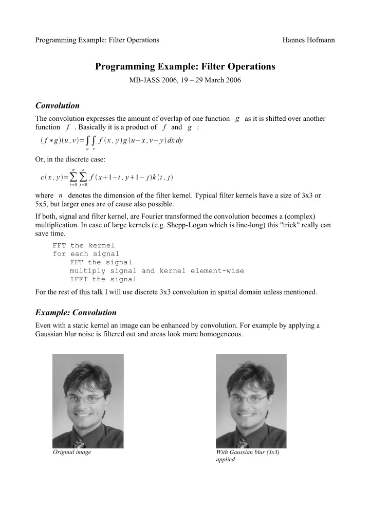
Programming Example: Filter Operations Hannes Hofmann Programming Example: Filter Operations MB-JASS 2006, 19 – 29 March 2006 Convolution The convolution expresses the amount of overlap of one function g as it is shifted over another f . Basically it is a product of f and g : function f ∗ g u ,v = ∫ u ∫ f x , y g u − x ,v − y dx dy v Or, in the discrete case: n n c x , y = ∑ ∑ f x 1 − i , y 1 − j k i , j i = 0 j = 0 where n denotes the dimension of the filter kernel. Typical filter kernels have a size of 3x3 or 5x5, but larger ones are of cause also possible. If both, signal and filter kernel, are Fourier transformed the convolution becomes a (complex) multiplication. In case of large kernels (e.g. Shepp-Logan which is line-long) this "trick" really can save time. FFT the kernel for each signal FFT the signal multiply signal and kernel element-wise IFFT the signal For the rest of this talk I will use discrete 3x3 convolution in spatial domain unless mentioned. Example: Convolution Even with a static kernel an image can be enhanced by convolution. For example by applying a Gaussian blur noise is filtered out and areas look more homogeneous. Original image With Gaussian blur (3x3) applied
Programming Example: Filter Operations Hannes Hofmann Furthermore one can extract valuable information out of images, e.g. edge information. Original image With horizontal Sobel With vertical Sobel -1 -2 -1 -1 0 1 0 0 0 -2 0 2 1 2 1 -1 0 1 Border Conditions For each pixel we compute we need the values of the neighbouring pixels. For the border pixels not all neighbours exist, so we must define what values we will use in that case. The larger our kernel is the more pixels are missing. Zeros – Set all outer pixels to zero. Clamping – Use the value of the border pixel for all pixels that lie outside of the image. Wrapping – Take the value of the border pixel on the opposite side. Anything else – One may think of any other way to handle this problem, just make sure that you don't get undesired results. Partitioning The Local Store of our SPUs has only a capacity of 256 KB. Most real-world problems will not fit into that little storage. Furthermore we want to use more than just one SPU in parallel to reduce computation time. That is why we have to divide our problem into several smaller ones. Of course this implies an overhead and you have to decide if it's worth the effort. Each data block has its own borders e.g., so you may have to transfer more input date onto the SPUs than you get as result. And what happens if one subtask is much faster than another one? It would be a pitty if 7 out of 8 SPUs stall because they are waiting for the other one to finish.
Programming Example: Filter Operations Hannes Hofmann Partitioning: Strategies One partitioning strategy that is known from DSPs is the pipeline model. The problem is divided into several subsequent sub-problems. Each of these is then assigned to one SPU that solves it and sends its results to the next SPU. Typically you don't want to do that on the Cell because you have to make sure that each stage of the pipeline takes approx. Equally long to avoid stalls.. A model that better fits to the CBEA is a static partitioning of the task. Basically you divide your input (or output) data into N blocks and send one to each of your SPUs, wait for all the results and send the next blocks. That way you can be sure that every SPU has about the same amount of work. In the case that you want some SPUs to do a different task you will run into troubles again, so you may want to use a more flexible scheduling algorithm. For example an SPU signals the PPU when it has finished its task and the PPU then gives the next workload to it. IBM has also introduced an advanced programming model called the microtask model in which the compiler assists the programmer in partitioning. Every block in the code is a microtask and as many mircotask as possible make an SPU task. Scalar Code The scalar convolution code is fairly simple. Just iterate over all pixels and sum up the products of all neighbours and the corresponding kernel element: for each line for each column as col for (k=0; k<3; ++k) { out[line][col] += in[line][col+k] * kern[k] out[line][col] += in[line+1][col+k] * kern[k+3] out[line][col] += in[line+2][col+k] * kern[k+6] } Note: the input image is larger than the output image here (see Border Conditions). 3x3 Convolution from IBM's sample library The scalar code performs very bad on the Cell hardware, because it benefits from none of its performance improving features. Fortunately IBM supplies us with an optimized convolution that exploits the architcture. void _conv3x3_1f (const float *in[3], float *out, const vec_float4 m[9], int w) { // init local variables const vec_float4 *in0 = (const vec_float4 *)in[0]; // ... in2 vec_float4 m00 = m[0]; // ... m08 // pre-process // init some pointers to handle left border (_CLAMP_CONV, // _WRAP_CONV)
Programming Example: Filter Operations Hannes Hofmann // process the line for (i0=0, i1=1, i2=2, i3=3, i4=4; i0<(w>>2)-4; i0+=4, i1+=4, i2+=4, i3+=4, i4+=4) { res = resu = resuu = resuuu = VEC_SPLAT_F32(0.0f); _GET_SCANLINE_x4(p0, in0[i0], in0[i1], in0[i2], in0[i3], in0[i4]); _CONV3_1f(m00, m01, m02); _GET_SCANLINE_x4(p1, in1[i0], in1[i1], in1[i2], in1[i3], in1[i4]); _CONV3_1f(m03, m04, m05); _GET_SCANLINE_x4(p2, in2[i0], in2[i1], in2[i2], in2[i3], in2[i4]); _CONV3_1f(m06, m07, m08); vout[i0] = res; vout[i1] = resu; vout[i2] = resuu; vout[i3] = resuuu; } // process line // post-process // right border } At first some local variables are initialized. Those *u , *uu and *uuu variables have the same semantics as prev , curr and next , but are used to unroll the computation by a factor of 4 #define _GET_SCANLINE_x4(_p, _a, _b, _c, _d, _e) \ prev = _p; \ curr = prevu = _a; \ next = curru = prevuu = _b; \ nextu = curruu = prevuuu = _c; \ nextuu = curruuu = _p = _d; \ nextuuu = _e next nextu, nextuu nextuuu curr, curru, curruu, curruuu prev prevu prevuu prevuuu 4 36 1 1 5 7 9 11 4 7 1 1 6 9 9 8 1 3 3 7 in[0]=in0
Programming Example: Filter Operations Hannes Hofmann _CONV3_1f is just a helper macro that calls others. #define _CONV3_1f(_m0, _m1, _m2) \ _GET_x4(prev, curr, left, left_shuf); \ _GET_x4(curr, next, right, right_shuf); \ _CALC_PIXELS_1f_x4(left, _m0, res); \ _CALC_PIXELS_1f_x4(curr, _m1, res); \ _CALC_PIXELS_1f_x4(right, _m2, res) Now it's time to visit the neighbours. shuf is a shuffle left or right by one pixel. #define _GET_x4(_a, _b, _c, _shuf) \ _c = vec_perm(_a, _b, _shuf); \ _c##u = vec_perm(_a##u, _b##u, _shuf); \ _c##uu = vec_perm(_a##uu, _b##uu, _shuf); \ _c##uuu = vec_perm(_a##uuu, _b##uuu, _shuf) And finally: work! Now the products are computed and accumulated. #define _CALC_PIXELS_1f_x4(_a, _b, _c) \ _c = vec_madd(_a, _b, _c); \ _c##u = vec_madd(_a##u, _b, _c##u); \ _c##uu = vec_madd(_a##uu, _b, _c##uu); \ _c##uuu = vec_madd(_a##uuu, _b, _c##uuu) curr // in scalar terms: res += left * m0 + curr * m1 5 7 9 11 in0 + right * m2 1 5 7 9 left, leftu, 7 9 11 4 right, rightu, The engineers at IBM did several optimizations of the scalar code. 1. Vectorization to exploit SIMD By using the left and right variables in addition to the curr vector 4 pixels can be computed at the same time. All arithmetic instructions work on vectors of 4 floats (vec_madd). The possible speedup thereof is 4. 2. Loop-unrolling to avoid stalls Those *u , *uu and *uuu variables allow the compiler to do a better scheduling of arithmetic and Load/Store/Shuffle operations on the two pipelines. This can improve the dual issue rate and reduce stalls. Another specialty of IBM's code is that it runs on VMX and SPU, just by switching the compiler.
Recommend


More recommend
Explore More Topics
Stay informed with curated content and fresh updates.