Extending the linear model DAAG Chapters 7 and 8 Learning - PowerPoint PPT Presentation
Extending the linear model DAAG Chapters 7 and 8 Learning objectives The linear model framework can be extended in many ways. We will learn about Indicator variables for coding factors Fitting multiple lines Polynomial regression
Extending the linear model DAAG Chapters 7 and 8
Learning objectives The linear model framework can be extended in many ways. We will learn about ◮ Indicator variables for coding factors ◮ Fitting multiple lines ◮ Polynomial regression ◮ Splines We will also learn about generalized linear models (glm) ◮ How the glm differs ◮ Logistic regression ◮ Ordinal regression ◮ Poisson regression
The linear model framework The multiple linear regression model can be written y = X β + ǫ where the distribution for the ǫ ’s is iid Normal. Critically important is the design matrix X ◮ Including an intercept ◮ Coding factors (multiple intercepts) ◮ Coding interactions (multiple slopes) ◮ Polynomial regression ◮ Splines
Coding factors (separate intercepts) ◮ Factors are categorical variables that may or may not be ordered. ◮ In the design matrix, we code factors using 1’s and 0’s ◮ For example, if we have a factor for eye colour (blue, brown, other), and the data are: blue, blue, brown, other, brown, other, blue, brown, blue 1 0 0 1 1 0 1 0 0 1 1 0 1 1 0 1 0 1 1 0 1 1 − 1 − 1 X = 1 1 0 X = 1 0 1 1 0 1 1 − 1 − 1 1 0 0 1 1 0 1 1 0 1 0 1 1 0 0 1 1 0 Treatment contrasts Sum (to zero) contrasts
Coding interactions (separate slopes) ◮ For a data set with: ◮ Continuous response y ◮ One three-level factor explanatory variable z ◮ One continuous explanatory variable x What models are available? 1. y = β 0 (constant) 2. y = β 0 + β 1 x (single line) 3. y = β 01 + β 02 z 2 + β 03 z 3 (three constants) 4. y = β 01 + β 02 z 2 + β 03 z 3 + β 1 x (three parallel lines) 5. y = β 01 + β 02 z 2 + β 03 z 3 + β 11 x + β 12 z 2 x + β 13 z 3 x (three separate lines) 6. y = β 0 + β 11 x + β 12 z 2 x + β 13 z 3 x (three lines, one intercept)
Polynomial regression ◮ Polynomials provide a simple way to model curved relationships ◮ Sometimes there is a good theoretical reason to use a polynomial relationship ◮ Including higher order terms directly in the design matrix is one option ◮ Orthogonal polynomials are a good alternative because the correlation between model coefficients will be zero ◮ this means greater numerical stability ◮ lower-order coefficients won’t change if higher-order coefficients are removed from the model ◮ In R, use poly() to specify orthogonal polynomials in a formula argument ◮ In SAS, use ORPOL function in PROC IML to generate design matrix columns
Splines ◮ Splines extend the idea of polynomial regression ◮ We do polynomial regression, but piecewise, joining the pieces at knots y = β 0 P 0 ( x ) + β 1 P 1 ( x ) + . . . + β k P k ( x ) ◮ The P i ( x ) are basis functions. They are polynomial functions that are sometimes constrained to be non-zero for only certain values of x . ◮ Two possible choices for P i ( x ) are B-splines and natural splines (linear beyond the data). ◮ By adding an error term, these spline functions can be fit using the linear model framework ◮ P i ( x ) is computed for all x in the data and all i ◮ These P i ( x ) make up the design matrix in the linear model fit
Splines A: N−spline, 1 internal knots (d.f. = 2+1) B: N−spline, 2 internal knots (d.f. = 3+1) 10000 10000 ● ● ● ● ● ● Resistance (ohms) ● ● ● ● ● ● ● ● ● ● ● ● ● ● ● ● ● ● ● ● ● ● ● ● ● ● ● ● ● ● ● ● ● ● 6000 ● ● ● ● ● ● 6000 ● ● ● ● ● ● ● ● ● ● ● ● ● ● ● ● ● ● ● ● ● ● ● ● ● ● ● ● ● ● ● ● ● ● ● ● ● ● ● ● ● ● ● ● ● ● ● ● ● ● ●● ● ● ● ●● ● ● ● ● ● ● ● ● ● ● ● ● ● ● ● ● ● ● ● ● ● ● ● ● ● ● ● ● ● ● ● ● ● ● ● ● ● ● ● ● ● ● ● ● ● ● ● ● ● ● ● ● ● ● ● ● ● ● ● ● ● ● ● ● ● ● ● ● ● ● ● ● ● ● ● ● ● ● ● ● ● ● ● ● ● ● ● ● ● ● ● ● ● ● ● ● ● ● ● ● ● ● ● ● ● ● ● ● ● ● ● ● ● 2000 ● ● ● ● ●● 2000 ● ● ● ● ●● ● ● ● ● ● ● ● ● ● ● ● ● ● ● ● ● ● ● ● ● ● ● ● ● ● ● ● ● 10 20 30 40 50 60 10 20 30 40 50 60
Splines A: Degree 2 N−spline B: Degree 3 N−spline ● −2105 ● −2569 Intercept = 8041 Intercept = 7569 ● ● ● ● 0.6 Spline basis functions 0.6 ● ● ● ● ● ● ● ● ● ● ● ● ● ● ● ● ● ● ● ● ● ● ●● ● ● ● ● ● ● ● ● ● ● ● ● ● ● ● ● ● ● ● ● ● ● ● ●● ● ● ● ● ● ● ● ●● ● ● ● ● ● ● ● ● ● ● ● ● ● ● ● ● ● ● ● ● ● ● ● −6329 ● ● ● ● ● 0.4 ● ● ● ● ● ● ● ● ● 0.4 ●● ● ● ● ● ● ● ● ● −8596 ● ● ● ● ● ● ● ● ● ● ● ● ● ● ● ● ● ● ● ● ● ● ● ● ● ● ● ● ● ● ● ● ● ● ● ● ● ● ● ● ● ● ● ● ● ● ● ● ● ● ● ● ● ● ● ● ● ● ● ● ● ● ● ● 0.2 ● ● ● ● ● ● ● 0.2 ● ● ● ● ● ● ● ● ● ● ● ● ● ● ● ● ● ● ● ● ● ● ● ● ● ● ● ● ● ● ● ● ● ● 0.0 ● ● ● ● ● ● ● ●● ● ● ● ● ● ● ● ●● ● ●● ● ● 0.0 ● ● ● ● ● ● ● ● ● ● ● ● ● ● ● ● ● ● ● ● ● ● ● ● ● ●● ● ● ● ● ● ● ● ● ● ● −4535 ● ● ● ● ● ● ● ● ● ● ● ● ● ● ● ● ● −0.2 ● ● ● ● ● ● ● ● ● ● ● ● ● ● ● ● ● ● ● ● ● −0.2 ● ● ● ● ● ● ●● ● ●● ● ● ● ● ● ●● ●● ● ● ● ● ● ● ● ● ● ● ● ● ● ● ● ● −0.4 7000 Fitted curve (ohms) 7000 5000 5000 3000 3000 10 20 30 40 50 60 10 20 30 40 50 60 Apparent juice content Apparent juice content
Generalized linear models GLMs extend the linear modelling framework by allowing ◮ Non-Gaussian errors ◮ A link function that transforms the linear model response The linear models we have considered so far had the form y = X β + ǫ, ǫ iid ∼ N (0 , σ 2 ) E [ y ] = X β The generalized linear model is f ( E [ y ]) = X β where f () is the link function. Also y = E [ y ] + ǫ or y ∼ ( E [ y ] , θ ) but here ǫ can have a non-Gaussian distribution.
Logistic regression In binomial logistic regression, the errors are binomial and the link function is logistic � E [ y ] � f ( E [ y ]) = log 1 − E [ y ] In this context, the E [ y ] = p , the binomial probability. The model for E [ y ] is � p � f ( p ) = log = X β 1 − p or exp( X β ) p = 1 + exp( X β ) and y ∼ Binom ( n , p ), or y ∼ Bern ( p ). ◮ Fit by maximizing likelihood of y as a function of β . ◮ Model comparison via deviance ( − 2 log L ( y | ˆ β )). ◮ Confidence intervals for β using the likelihood.
Ordinal regression ◮ Ordinal response, link is usually logistic ◮ Here we look at the cumulative probabilities γ j = P ( y ≤ j ) � γ j � log = η j − X β 1 − γ j ◮ The η j are cutpoints between the response categories η i < η j for i < j ◮ Assumption: β -effects are proportional to the odds for all j = exp( η j ) 1 − γ j γ j or = exp( X β ) exp( − η j ) 1 − γ j exp( X β ) γ j ◮ Or, can include separate β j for each j .
Poisson regression ◮ Errors are Poisson, link function most commonly log ◮ Recall that Poisson is for count data that arise from a Poisson process ◮ E [ y ] = λ , the rate parameter. The model is f ( λ ) = log( λ ) = X β or E [ y ] = λ = exp( X β ) and y ∼ Poisson ( λ ). ◮ Note that the Poisson distribution has Var ( y ) = λ . If we have over- or under- dispersion, we can relax this requirement and estimate a dispersion parameter φ (quasipoisson).
Example: Head injuries ◮ Data: (simulated) patient data that present with head injuries ◮ Q: Can we identify patients that would be classified as high risk using available criteria? ◮ Response: Whether a patient is classified as high risk by a clinician ◮ Explanatory variables: ◮ Whether over age 65 ◮ Amount of amnesia before impact (threshold 30 mins) ◮ Basal skull fracture present ◮ Open skull fracture present ◮ Whether vomiting ◮ Whether loss of consciousness occurred ◮ Use logistic regression
Recommend
More recommend
Explore More Topics
Stay informed with curated content and fresh updates.

