Exponentially Weighted Moving Average Chart Given a sequence of - PowerPoint PPT Presentation
ST 435/535 Statistical Methods for Quality and Productivity Improvement / Statistical Process Control Exponentially Weighted Moving Average Chart Given a sequence of observations x 1 , x 2 , . . . , x n , the e xponentially w eighted m oving a
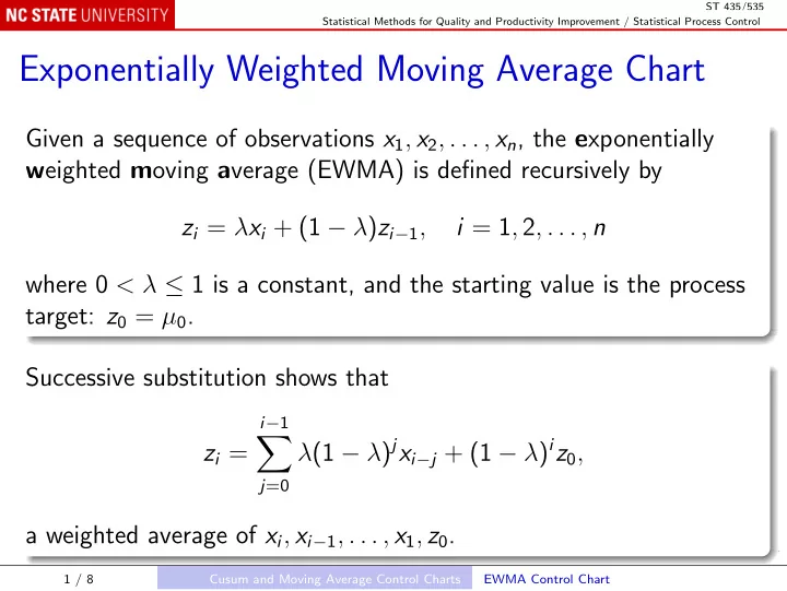
ST 435/535 Statistical Methods for Quality and Productivity Improvement / Statistical Process Control Exponentially Weighted Moving Average Chart Given a sequence of observations x 1 , x 2 , . . . , x n , the e xponentially w eighted m oving a verage (EWMA) is defined recursively by z i = λ x i + (1 − λ ) z i − 1 , i = 1 , 2 , . . . , n where 0 < λ ≤ 1 is a constant, and the starting value is the process target: z 0 = µ 0 . Successive substitution shows that i − 1 � λ (1 − λ ) j x i − j + (1 − λ ) i z 0 , z i = j =0 a weighted average of x i , x i − 1 , . . . , x 1 , z 0 . 1 / 8 Cusum and Moving Average Control Charts EWMA Control Chart
ST 435/535 Statistical Methods for Quality and Productivity Improvement / Statistical Process Control So if E( X i ) = µ 0 , then E( Z i ) = µ 0 , and if the observations X i are uncorrelated random variables with variance σ 2 , then � � � λ Var( Z i ) = σ 2 1 − (1 − λ ) 2 i � . 2 − λ We can set up an L -sigma control chart for z i : �� � λ [1 − (1 − λ ) 2 i ] UCL = µ 0 + L σ 2 − λ Center line = µ 0 �� � λ [1 − (1 − λ ) 2 i ] LCL = µ 0 − L σ 2 − λ 2 / 8 Cusum and Moving Average Control Charts EWMA Control Chart
ST 435/535 Statistical Methods for Quality and Productivity Improvement / Statistical Process Control In R: Use the simulated data used as an example of the cusum chart; recall that µ 0 = 10 and σ = 1; use λ = 0 . 1 and L = 2 . 7: library(qcc) summary(ewma(x, center = 10, std.dev = 1, lambda = 0.1, nsigmas = 2.7)) Notes The control limits change with i , but approach asymptotes. The same two observations fall outside the control limits as in the Cusum control chart. 3 / 8 Cusum and Moving Average Control Charts EWMA Control Chart
ST 435/535 Statistical Methods for Quality and Productivity Improvement / Statistical Process Control Design Like the cusum chart, the EWMA chart’s properties are difficult to calculate, so the focus is on the ARL. The performance of the chart is determined by L and λ . Suppose we want an EWMA chart with a specified ARL 0 , say 370, and a low ARL 1 for a one-sigma shift. For any choice of λ , the function xewma.crit(l, L0) in the spc package computes the L that gives the desired ARL 0 , L0 , for a given λ , l . 4 / 8 Cusum and Moving Average Control Charts EWMA Control Chart
ST 435/535 Statistical Methods for Quality and Productivity Improvement / Statistical Process Control Optimal design o <- optimize(function(lambda) xewma.arl(l = lambda, c = xewma.crit(lambda, 370, sided = "two"), mu = 1, sided = "two"), interval = c(0, 1)) print(o) xewma.crit(o$minimum, 370, sided = "two") The optimal λ = 0 . 14 and control limits L = 2 . 79, with ARL 1 = 9 . 58. The performance is very similar to, but slightly better than, the optimal cusum chart (with no head start), for which the ARL 1 was 9.92. 5 / 8 Cusum and Moving Average Control Charts EWMA Control Chart
ST 435/535 Statistical Methods for Quality and Productivity Improvement / Statistical Process Control Moving Average Control Chart The EWMA chart is easy to set up recursively, since the current value of z depends on only the current x and the previous z . However, because it is a (exponentially) weighted average of all past observations, it is impacted, at least a little, by the entire past. An alternative, with finite memory, is the m oving a verage (MA) chart with span w , based on the unweighted average m i = x i + x i − 1 + · · · + x i − w +1 i = w , w + 1 , . . . . w 6 / 8 Cusum and Moving Average Control Charts Moving Average Control Chart
ST 435/535 Statistical Methods for Quality and Productivity Improvement / Statistical Process Control For i < w , we define m i to be the average of x 1 , x 2 , . . . , x i . If E( X i ) = µ 0 and the X s are uncorrelated with variance σ 2 , then E( M i ) = µ 0 , and σ 2 Var( M i ) = min( w , i ) 7 / 8 Cusum and Moving Average Control Charts Moving Average Control Chart
ST 435/535 Statistical Methods for Quality and Productivity Improvement / Statistical Process Control So we can construct a control chart for m i with � 1 UCL = µ 0 + L σ min( w , i ) Center line = µ 0 � 1 LCL = µ 0 − L σ min( w , i ) Like the EWMA chart, the limits change with i , but are constant after i ≥ w , instead of asymptoting to a constant. See Figure 9.8; the qcc package does not provide MA control charts. 8 / 8 Cusum and Moving Average Control Charts Moving Average Control Chart
Recommend
More recommend
Explore More Topics
Stay informed with curated content and fresh updates.
