Explicit Characterisation of Receding Horizon Control Mar a M. - PowerPoint PPT Presentation
Explicit Characterisation of Receding Horizon Control Mar a M. Seron September 2004 Centre for Complex Dynamic Systems and Control Outline Solution Using Geometry 1 Solution for Arbitrary N Example Implementation of the Explicit
Explicit Characterisation of Receding Horizon Control Mar´ ıa M. Seron September 2004 Centre for Complex Dynamic Systems and Control
Outline Solution Using Geometry 1 Solution for Arbitrary N Example Implementation of the Explicit Solution 2 Calculation of the Explicit Solution On-line Implementation of the Explicit Solution Suboptimal Solutions and Approximations Centre for Complex Dynamic Systems and Control
The Receding Horizon Optimal Control Problem Let the system be given by x k + 1 = Ax k + Bu k , | u k | ≤ ∆ , (1) where x k ∈ R n and ∆ > 0 is the input constraint level. Consider the following fixed horizon optimal control problem V P 2 ( x ) : 2 ( x ) � min V 2 ( { x k } , { u k } ) , (2) subject to: x k + 1 = Ax k + Bu k for k = 0 , 1 , x 0 = x , u k ∈ U � [ − ∆ , ∆ ] for k = 0 , 1 , where the objective function in (2) is 1 V 2 ( { x k } , { u k } ) � 1 2 Px 2 + 1 � � � 2 x x k Qx k + u k Ru k . (3) 2 k = 0 Centre for Complex Dynamic Systems and Control
The Receding Horizon Optimal Control Problem In the objective function we select Q > 0, R > 0 and P satisfying the algebraic Riccati equation P = A PA + Q − K ¯ RK , (4) where K � ¯ R − 1 B PA , ¯ R � R + B PB . (5) Let the control sequence that minimises (3) be { u 0 , u 1 } . (6) Then the RHC law is given by the first element of (6) (which depends on the current state x 0 = x ), that is, K 2 ( x ) = u 0 . (7) Centre for Complex Dynamic Systems and Control
Solution of the Associated QP In the previous lecture we showed that the solution in active region R 8 is � − Gx − h � u ( x ) = ∆ where G = K + KBKA KB h = 1 + ( KB ) 2 ∆ , 1 + ( KB ) 2 if [ 0 1 ] u ( x ) ≥ ∆ R 8 : H 1 ∆ [ − 1 1 ] ≤ [ 1 0 ] H u ( x ) ≤ H 1 ∆ [ 1 1 ] ( x ) = − H − 1 Fx . where u Centre for Complex Dynamic Systems and Control
Solution of the Associated QP ( x ) = − H − 1 Fx belongs to The above solution is valid whenever u R 8 , that is, it satisfies the equations [ 0 1 ] u ≥ ∆ R 8 : H 1 ∆ [ − 1 1 ] ≤ [ 1 0 ] H u ≤ H 1 ∆ [ 1 1 ] . ( x ) = − H − 1 Fx in the above equations we Thus, setting u = u obtain a characterisation of R 8 in the state space: − [ 0 1 ] H − 1 Fx ≥ ∆ R 8 : H 1 ∆ [ − 1 1 ] ≤ − [ 1 0 ] Fx ≤ H 1 ∆ [ 1 1 ] . Centre for Complex Dynamic Systems and Control
Geometric RHC Characterisation for N = 2 If we proceed in a similar way with the remaining regions, we obtain a characterisation of the RHC law in the form 4 R 3 R 4 3 R 5 − Kx if x ∈ R , 2 R 2 ∆ if x ∈ R 1 ∪ R 2 ∪ R 3 , 1 x 2 k R 0 K 2 ( x ) = − Gx + h if x ∈ R 4 , −1 − ∆ if x ∈ R 5 ∪ R 6 ∪ R 7 , R 6 −2 R 1 − Gx − h if x ∈ R 8 , −3 R 8 R 7 −4 −8 −6 −4 −2 0 2 4 6 8 x 1 k where the regions R , R 1 , . . . , R 8 in the state space are obtained using geometric arguments as described before. We can see that the above characterisation coincides with the one obtained previously using Dynamic Programming. Centre for Complex Dynamic Systems and Control
Geometric RHC Characterisation. More General Cases For arbitrary horizon N , m ≥ 1 inputs, and more general constraints, as we showed in the previous lecture, the QP solution in a particular active region corresponding to the face Φ ℓ u = ∆ ℓ − Λ ℓ x , has the form u ( x ) = H − 1 / 2 ˜ ℓ [ ˜ Φ ℓ ˜ ℓ ] − 1 ( ∆ ℓ − Λ ℓ x ) Φ Φ ℓ ] − 1 ˜ − H − 1 / 2 [ I − ˜ Φ ℓ ] H − 1 / 2 Fx , ℓ [ ˜ Φ ℓ ˜ Φ Φ � G ℓ x + h ℓ . Centre for Complex Dynamic Systems and Control
Geometric RHC Characterisation. More General Cases The above QP solution is valid in the state space region L ℓ x ≤ W ℓ , where [ ˜ Φ ℓ ˜ ℓ ] − 1 ( Λ ℓ − ˜ � Φ ℓ H − 1 / 2 F ) � Φ L ℓ = Φ s ˜ ˜ ℓ [ ˜ Φ ℓ ˜ ℓ ] − 1 ( Λ ℓ − ˜ Φ ℓ H − 1 / 2 F ) + ( Λ s − ˜ Φ s H − 1 / 2 F ) Φ Φ [ ˜ Φ ℓ ˜ ℓ ] − 1 ∆ ℓ � � Φ W ℓ = ∆ s + ˜ Φ s ˜ ℓ [ ˜ Φ ℓ ˜ ℓ ] − 1 ∆ ℓ Φ Φ Centre for Complex Dynamic Systems and Control
Geometric RHC Characterisation. More General Cases Thus, the optimal QP solution in an active region (corresponding to active constraints with indices in ℓ ) is u ( x ) � G ℓ x + h ℓ , whenever x satisfies L ℓ x ≤ W ℓ . The RHC law K N ( x ) in the above region is then given by the first m elements of the above solution: K N ( x ) = [ I m 0 ]( G ℓ x + h ℓ ) if L ℓ x ≤ W ℓ . (8) Centre for Complex Dynamic Systems and Control
Geometric RHC Characterisation. More General Cases To compute the complete RHC solution in the state space one requires, for example, procedures that enumerate all combinations of active constraints, or recursively partition the state space searching for active regions, or enumerate all parameterised vertices based on double description properties of polyhedra. We will briefly comment on these computational issues later. Centre for Complex Dynamic Systems and Control
Example Consider a system with matrices � � � � 0 . 8955 − 0 . 1897 0 . 0948 A = , B = . 0 . 0948 0 . 9903 0 . 0048 � � 0 0 In the objective function we take N = 4, Q = and R = 0 . 01. 0 2 The terminal state weighting matrix P is chosen as the solution of the algebraic Riccati equation P = A PA + Q − K ¯ RK , where K � ¯ R − 1 B PA and ¯ R � R + B PB . We consider input constraints of the form | u k | ≤ 2. Centre for Complex Dynamic Systems and Control
Example The state space partition for this case is shown in Figure (a). A “zoom” of this partition is shown in Figure (b). The region denoted by X 0 is the projection onto the state space of the constraint polyhedron; in regions X 2 , X 3 and X 4 only one constraint is active; in regions X 5 and X 6 two constraints are active; in region X 7 three constraints are active; finally, X 1 is the union of all regions where the control is saturated to the value − 2. 1 X 7 0.8 0.55 0.6 X X 6 0.5 6 X 4 0.4 0.45 X 7 0.2 x 2 0.4 x 2 X 0 0 X 3 X 0 0.35 −0.2 X 5 0.3 −0.4 X 1 0.25 X 1 X 2 −0.6 0.2 −0.8 −1 0.15 −2.5 −2 −1.5 −1 −0.5 0 0.5 1 1.5 2 −1.6 −1.5 −1.4 −1.3 −1.2 −1.1 −1 −0.9 x 1 x 1 (a) Complete partition. (b) Zoom. Centre for Complex Dynamic Systems and Control
Example The resulting RHC law (8) is K 4 ( x ) = G i x + h i , if x ∈ X i , i = 0 , . . . , 7 , (9) where G 0 = − [ 4 . 4650 13 . 5974 ] , h 0 = 0 , G 1 = [ 0 0 ] , h 1 = − 2 , G 2 = − [ 5 . 6901 15 . 9529 ] , h 2 = − 0 . 7894 , G 3 = − [ 4 . 9226 13 . 8202 ] , h 3 = − 0 . 4811 , G 4 = − [ 4 . 5946 13 . 3346 ] , h 4 = − 0 . 2684 , G 5 = − [ 6 . 6778 16 . 8644 ] , h 5 = − 1 . 7057 , G 6 = − [ 5 . 1778 13 . 4855 ] , h 6 = − 0 . 9355 , G 7 = − [ 7 . 4034 16 . 8111 ] , h 7 = − 2 . 6783 . Similar expressions hold in the remaining unlabelled regions. These can be obtained by symmetry. Centre for Complex Dynamic Systems and Control
Example The figures show the state state partitions for horizons N = 2, N = 3, N = 4 and N = 5. 1 1 N = 2 N = 3 0.8 0.8 0.6 0.6 0.4 0.4 0.2 0.2 x 2 x 2 0 0 −0.2 −0.2 −0.4 −0.4 −0.6 −0.6 −0.8 −0.8 −1 −1 −3 −2 −1 0 1 2 3 −3 −2 −1 0 1 2 3 x 1 x 1 1 1 N = 4 0.8 0.8 N = 5 0.6 0.6 0.4 0.4 0.2 0.2 x 2 x 2 0 0 −0.2 −0.2 −0.4 −0.4 −0.6 −0.6 −0.8 −0.8 −1 −1 −3 −2 −1 0 1 2 3 −3 −2 −1 0 1 2 3 x 1 x 1 Centre for Complex Dynamic Systems and Control
Example We next consider an initial condition x 0 = [ − 1 . 2 0 . 53 ] and simulate the system under the RHC (9). 0.6 The figure shows the resulting 0.5 state space trajectory. 0.4 The trajectory starts in region X 4 0.3 x 2 and moves, successively, into 0.2 regions X 6 , X 5 , X 1 , X 1 , X 0 , and 0.1 stays in X 0 thereafter. 0 −1.4 −1.2 −1 −0.8 −0.6 −0.4 −0.2 0 x 1 Centre for Complex Dynamic Systems and Control
Recommend


More recommend
Explore More Topics
Stay informed with curated content and fresh updates.