1 Inference and estimation in probabilistic time series models - PDF document

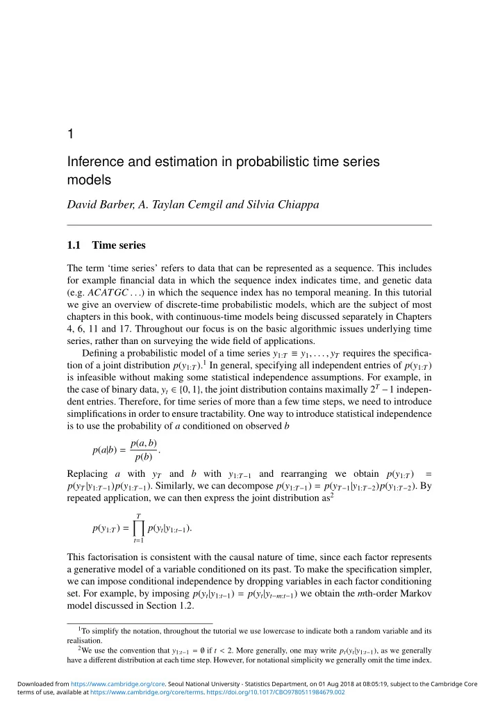
1 Inference and estimation in probabilistic time series models David Barber, A. Taylan Cemgil and Silvia Chiappa 1.1 Time series The term ‘time series’ refers to data that can be represented as a sequence. This includes for example financial data in which the sequence index indicates time, and genetic data (e.g. ACATGC . . . ) in which the sequence index has no temporal meaning. In this tutorial we give an overview of discrete-time probabilistic models, which are the subject of most chapters in this book, with continuous-time models being discussed separately in Chapters 4, 6, 11 and 17. Throughout our focus is on the basic algorithmic issues underlying time series, rather than on surveying the wide field of applications. Defining a probabilistic model of a time series y 1: T ≡ y 1 , . . . , y T requires the specifica- tion of a joint distribution p ( y 1: T ). 1 In general, specifying all independent entries of p ( y 1: T ) is infeasible without making some statistical independence assumptions. For example, in the case of binary data, y t ∈ { 0 , 1 } , the joint distribution contains maximally 2 T − 1 indepen- dent entries. Therefore, for time series of more than a few time steps, we need to introduce simplifications in order to ensure tractability. One way to introduce statistical independence is to use the probability of a conditioned on observed b p ( a | b ) = p ( a , b ) p ( b ) . Replacing a with y T and b with y 1: T − 1 and rearranging we obtain p ( y 1: T ) = p ( y T | y 1: T − 1 ) p ( y 1: T − 1 ). Similarly, we can decompose p ( y 1: T − 1 ) = p ( y T − 1 | y 1: T − 2 ) p ( y 1: T − 2 ). By repeated application, we can then express the joint distribution as 2 T � p ( y 1: T ) = p ( y t | y 1: t − 1 ) . t = 1 This factorisation is consistent with the causal nature of time, since each factor represents a generative model of a variable conditioned on its past. To make the specification simpler, we can impose conditional independence by dropping variables in each factor conditioning set. For example, by imposing p ( y t | y 1: t − 1 ) = p ( y t | y t − m : t − 1 ) we obtain the m th-order Markov model discussed in Section 1.2. 1 To simplify the notation, throughout the tutorial we use lowercase to indicate both a random variable and its realisation. 2 We use the convention that y 1: t − 1 = ∅ if t < 2. More generally, one may write p t ( y t | y 1: t − 1 ), as we generally have a di ff erent distribution at each time step. However, for notational simplicity we generally omit the time index. Downloaded from https://www.cambridge.org/core. Seoul National University - Statistics Department, on 01 Aug 2018 at 08:05:19, subject to the Cambridge Core terms of use, available at https://www.cambridge.org/core/terms. https://doi.org/10.1017/CBO9780511984679.002

2 David Barber, A. Taylan Cemgil and Silvia Chiappa y 1 y 2 y 3 y 4 y 1 y 2 y 3 y 4 (a) (b) Figure 1.1 Belief network representations of two time series models. (a) First-order Markov model p ( y 1:4 ) = p ( y 4 | y 3 ) p ( y 3 | y 2 ) p ( y 2 | y 1 ) p ( y 1 ). (b) Second-order Markov model p ( y 1:4 ) = p ( y 4 | y 3 , y 2 ) p ( y 3 | y 2 , y 1 ) p ( y 2 | y 1 ) p ( y 1 ). A useful way to express statistical independence assumptions is to use a belief network graphical model which is a directed acyclic graph 3 representing the joint distribution N � p ( y 1: N ) = p ( y i | pa ( y i )) , i = 1 where pa ( y i ) denotes the parents of y i , that is the variables with a directed link to y i . By limiting the parental set of each variable we can reduce the burden of specification. In Fig. 1.1 we give two examples of belief networks corresponding to a first- and second- order Markov model respectively, see Section 1.2. For the model p ( y 1:4 ) in Fig. 1.1(a) and binary variables y t ∈ { 0 , 1 } we need to specify only 1 + 2 + 2 + 2 = 7 entries, 4 compared to 2 4 − 1 = 15 entries in the case that no independence assumptions are made. Inference Inference is the task of using a distribution to answer questions of interest. For example, given a set of observations y 1: T , a common inference problem in time series analysis is the use of the posterior distribution p ( y T + 1 | y 1: T ) for the prediction of an unseen future variable y T + 1 . One of the challenges in time series modelling is to develop computationally e ffi - cient algorithms for computing such posterior distributions by exploiting the independence assumptions of the model. Estimation Estimation is the task of determining a parameter θ of a model based on observations y 1: T . This can be considered as a form of inference in which we wish to compute p ( θ | y 1: T ). Specifically, if p ( θ ) is a distribution quantifying our beliefs in the parameter values before having seen the data, we can use Bayes’ rule to combine this prior with the observations to form a posterior distribution p ( y 1: T | θ ) p ( θ ) � ��� �� ��� � ���� likelihood prior p ( θ | y 1: T ) = . p ( y 1: T ) � ��� �� ��� � posterior � � �� � � marginal likelihood The posterior distribution is often summarised by the maximum a posteriori (MAP) point estimate, given by the mode θ MAP = argmax p ( y 1: T | θ ) p ( θ ) . θ 3 A directed graph is acyclic if, by following the direction of the arrows, a node will never be visited more than once. 4 For example, we need one specification for p ( y 1 = 0), with p ( y 1 = 1) = 1 − p ( y 1 = 0) determined by normalisation. Similarly, we need to specify two entries for p ( y 2 | y 1 ). Downloaded from https://www.cambridge.org/core. Seoul National University - Statistics Department, on 01 Aug 2018 at 08:05:19, subject to the Cambridge Core terms of use, available at https://www.cambridge.org/core/terms. https://doi.org/10.1017/CBO9780511984679.002

Probabilistic time series models 3 It can be computationally more convenient to use the log posterior, θ MAP = argmax log ( p ( y 1: T | θ ) p ( θ )) , θ where the equivalence follows from the monotonicity of the log function. When using a ‘flat prior’ p ( θ ) = const. , the MAP solution coincides with the maximum likelihood (ML) solution θ ML = argmax p ( y 1: T | θ ) = argmax log p ( y 1: T | θ ) . θ θ In the following sections we introduce some popular time series models and describe associated inference and parameter estimation routines. 1.2 Markov models Markov models (or Markov chains) are of fundamental importance and underpin many time series models [21]. In an m th order Markov model the joint distribution factorises as T � p ( y 1: T ) = p ( y t | y t − m : t − 1 ) , t = 1 expressing the fact that only the previous m observations y t − m : t − 1 directly influence y t . In a time-homogeneous model, the transition probabilities p ( y t | y t − m : t − 1 ) are time-independent. 1.2.1 Estimation in discrete Markov models In a time-homogeneous first-order Markov model with discrete scalar observations y t ∈ { 1 , . . . , S } , the transition from y t − 1 to y t can be parameterised using a matrix θ , that is θ ji ≡ p ( y t = j | y t − 1 = i , θ ) , i , j ∈ { 1 , . . . , S } . Given observations y 1: T , maximum likelihood sets this matrix according to � θ ML = argmax log p ( y 1: T | θ ) = argmax log p ( y t | y t − 1 , θ ) . θ θ t Under the probability constraints 0 ≤ θ ji ≤ 1 and � j θ ji = 1, the optimal solution is given by the intuitive setting n ji θ ML = T − 1 , ji where n ji is the number of transitions from i to j observed in y 1: T . Alternatively, a Bayesian treatment would compute the parameter posterior distribution � n ji p ( θ | y 1: T ) ∝ p ( θ ) p ( y 1: T | θ ) = p ( θ ) θ ji . i , j In this case a convenient prior for θ is a Dirichlet distribution on each column θ : i with hyperparameter vector α : i 1 � � � α ji − 1 p ( θ ) = DI ( θ : i | α : i ) = θ , ji Z ( α : i ) i i j Downloaded from https://www.cambridge.org/core. Seoul National University - Statistics Department, on 01 Aug 2018 at 08:05:19, subject to the Cambridge Core terms of use, available at https://www.cambridge.org/core/terms. https://doi.org/10.1017/CBO9780511984679.002