Excursion 5 Tours I & II: Power: Pre-data, Post-data & How - - PowerPoint PPT Presentation

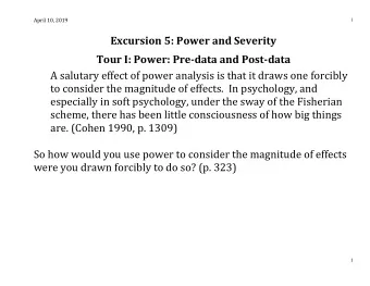
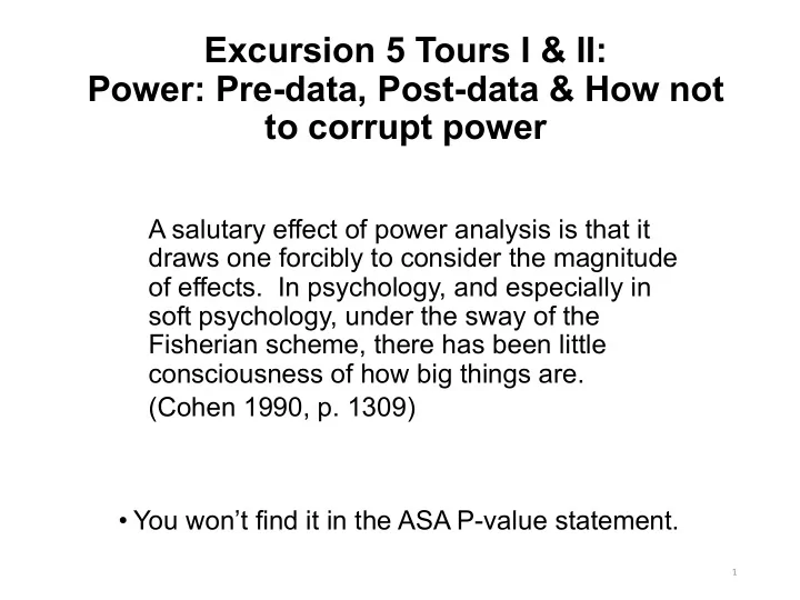
Excursion 5 Tours I & II: Power: Pre-data, Post-data & How not to corrupt power

A salutary effect of power analysis is that it draws one forcibly to consider the magnitude

• f effects. In psychology, and especially in

soft psychology, under the sway of the Fisherian scheme, there has been little consciousness of how big things are. (Cohen 1990, p. 1309)

• You won’t find it in the ASA P-value statement.

1

2

• Power is one of the most abused notions in all
• f statistics (we’ve covered it, but are doing a

bit more today)

• Power is always defined in terms of a fixed cut-
• ff cα, computed under a value of the

parameter under test These vary, there is really a power function.

• The power of a test against μ’, is the probability

it would lead to rejecting H0 when μ = μ’. (3.1) POW(T, μ’) = Pr(d(X) > cα; μ = μ’)

3

Fisher talked sensitivity, not power:

Oscar Kempthorne (being interviewed by J. Leroy Folks (1995)) said (SIST 325): “Well, a common thing said about [Fisher] was that he did not accept the idea of the

• power. But, of course, he must have.

However, because Neyman had made such a point abut power, Fisher couldn’t bring himself to acknowledge it” (p. 331).

4

Errors in Jacob Cohen’s definition in his Statistical Power Analysis for the Behavioral Sciences (SIST p. 324) Power: POW(T, μ’) = Pr(d(X) > cα; μ = μ’)

• Keeping to the fixed cut-off cα is too coarse for

the severe tester—but we won’t change the definition of power “

5

N-P gave three roles to power:

• first two are pre-data, for planning,

comparing tests; the third for interpretation post-data—to be explained in a minute (Hidden Neyman files, from R. Giere collection). Mayo and Spanos (2006, p. 337)

5.1 Power Howlers, Trade-offs and Benchmarks

Power is increased with increased n, but also by computing it in relation to alternatives further and further from the null.

• Example. A test is practically guaranteed to

reject H0, the “no improvement” null, if in fact H1 the drug cures practically everyone. (SIST p. 326)

6

7

It has high power to detect H1 But you wouldn’t say that its rejecting H0 is evidence H1 cures everyone. To think otherwise is to commit the second form of MM fallacy (p. 326) “This is a surprisingly widespread piece of nonsense which has even made its way into

• ne book on drug industry trials” (ibid., p.

201). (bott SIST, 328)

Trade-offs and Benchmarks

• a. The power against H0 is α.

POW(T+, μ0 ) = Pr( ! 𝑌 > ̅ 𝑦!; μ0), ̅ 𝑦! = (μ0 + zα𝜏 "

#),

𝜏 $

# = [σ/√n])

The power at the null is: Pr(Z > zα;μ0) = α. It’s the low power against H0 that warrants taking a rejection as evidence that μ > μ0 . We infer an indication of discrepancy from H0 because a null world would probably have yielded a smaller difference than observed.

8

9

• b. The power > .5 only for alternatives that

exceed the cut-off ̅ 𝑦!, Remember ̅ 𝑦! is (μ0 + zα𝜏 "

#).

The power of test T+ against μ = ! x% is .5. In test T+ the range of possible values of ! 𝑌 and µ are the same, so we are able to set µ values this way, without confusing the parameter and sample spaces.

10

An easy alternative to remember with reasonable high power (SIST 329): μ.84 : Abbreviation: the alternative against which test T+ has .84 power by μ.84 : The power of test T+ to detect an alternative that exceeds the cut-off ̅ 𝑦! by 1𝜏 "

# =.84.

Other shortcuts on SIST p. 328

Trade-offs Between α, the Type I Error Probability and Power

As the probability of a Type I error goes down the probability of a Type II error goes up (power goes down). If someone said: As the power increases, the probability

• f a Type I error decreases, they’d be saying, as the Type

II error decreases, the probability of a Type I error decreases. That’s the opposite of a trade-off! So they’re either using a different notion or are wrong about power. Many current reforms do just this!

11

12

Criticisms that lead to those reforms also get things backwards Ziliak and McCloskey “refutations of the null are trivially easy to achieve if power is low enough or the sample is large enough” (2008a, p. 152)? They would need to say power is high enough raising the power is to lower the hurdle, they get it backwards (SIST p. 330) More howlers on p. 331

Power analysis arises to interpret negative results: d(x0) ≤ cα:

• A classic fallacy is to construe no evidence

against H0 as evidence of the correctness of H0.

• “Researchers have been warned that a

statistically nonsignificant result does not ‘prove’ the null hypothesis (the hypothesis that there is no difference between groups or no effect of a treatment …)”. Amhrein et al., (2019) take this as grounds to “Retire Statistical Significance”

• No mention of power, designed to block this

fallacy

13

14

It uses the same reasoning as significance tests. Cohen: [F]or a given hypothesis test, one defines a numerical value i (or iota) for the [population] ES, where i is so small that it is appropriate in the context to consider it negligible (trivial, inconsequential). Power (1 – β) is then set at a high value, so that β is relatively small. When, additionally, α is specified, n can be found. Now, if the research is performed with this n and it results in nonsignificance, it is proper to conclude that the population ES is no more than i, i.e., that it is negligible… (Cohen 1988, p. 16; α, β substituted for his a, b).

15

Ordinary Power Analysis: If data x are not statistically significantly different from H0, and the power to detect discrepancy γ is high, then x indicates that the actual discrepancy is no greater than γ

Neyman an early power analyst

In his “The Problem of Inductive Inference” (1955) where he chides Carnap for ignoring the statistical model (p. 341). “I am concerned with the term ‘degree of confirmation’ introduced by Carnap. …We have seen that the application of the locally best one-sided test to the data…failed to reject the hypothesis [that the 26

• bservations come from a source in which the

null hypothesis is true]”.

16

17

“Locally best one-sided Test T A sample X = (X1, …,Xn) each Xi is Normal, N(μ,σ2), (NIID), σ assumed known; X ̅ the sample mean H0: μ ≤ μ0 against H1: μ > μ0. Test Statistic d(X) = (X ̅ - μ0)/σx, σx = σ /√𝑜 Test fails to reject the null, d(x0) ≤ cα. “The question is: does this result ‘confirm’ the hypothesis that H0 is true [of the particular data set]? ” (Neyman). Carnap says yes…

18

Neyman: “….the attitude described is dangerous. …the chance of detecting the presence [of discrepancy γ from the null], when only [this number] of observations are available, is extremely slim, even if [γ is present].” “One may be confident in the absence [of that discrepancy only] if the power to detect it were high”. (power analysis) If Pr(d(X) > cα; μ = μ0 + γ) is high d(X) ≤ cα; infer: discrepancy < γ

Problem: Too Coarse

Consider test T+ (α = .025): H0: μ = 150 vs. H1: μ ≥ 150, α = .025, n = 100, σ = 10, 𝜏 "

# = 1.

The cut-off = 152. Say ̅ 𝑦& = 151.9, just missing 152 Consider an arbitrary inference μ < 151. We know POW(T+, μ = 151) = .16 (1𝜏 "

# is

subtracted from 152). .16 is quite lousy power. It follows that no statistically insignificant result can warrant μ< 151 for the power analyst.

19

20

We should take account of the actual result: SEV(T+, ̅ 𝑦& = 149, μ < 151) = .975. Z = (149 -151)/1 = -2 SEV (μ < 151) = Pr (Z > z0; μ = 1) = .975

21

(1) P(d(X) > cα; μ = μ0 + γ) Power to detect γ

• Just missing the cut-off cα is the worst case
• It is more informative to look at the probability of

getting a worse fit than you did (2) P(d(X) > d(x0); μ = μ0 + γ) “attained power” Π(γ) Here it measures the severity for the inference μ < μ0 + γ Not the same as something called “retrospective power” or “ad hoc” power!

22

The only Time Severity equals Power for a claim

! 𝑌 just misses ̅ 𝑦! and you want SEV(μ < μ’) Then it equals POW(μ’) For claims of form μ > μ’ it’s the reverse: (the ex on p. 344 has different numbers but the point is the same)

Po Power vs Severity fo for 𝛎 > 𝛎𝟐

23

24

Severity for (nonsignificant results) and confidence bounds

Test T+: H0: μ < μ0 vs H1: μ > μ0 σ is known (SEV): If d(x) is not statistically significant, then test T+ passes µ < M0 + kεσ/ n.5 with severity ( 1 – ε), where P(d(X) > kε) = ε. The connection with the upper confidence limit is obvious.

25

One can consider a series of upper discrepancy bounds… SEV(μ < ̅ 𝑦& + 0σx) = .5 SEV(μ < ̅ 𝑦& + .5σx) = .7 SEV(μ < ̅ 𝑦& + 1σx) = .84 SEV(μ < ̅ 𝑦& + 1.5σx) = .93 SEV(μ < ̅ 𝑦& + 1.96σx) = .975 This relates to work on confidence distributions. But aren’t I just using this as another way to say how probable each claim is?

26

• No. This would lead to inconsistencies

(famous fiducial feuds) (Excursion 5 Tour III: Deconstructing N-P vs Fisher debates

27

The reasoning instead is counterfactual: H: μ < ̅ 𝑦& + 1.96σx (i.e., μ < CIu ) H passes severely because were this inference false, and the true mean μ > CIu then, very probably, we would have observed a larger sample mean

28

Power vs Severity analysis for non-significant results

Power Analysis (ordinary): If Pr(d(X) > cα; µ’) = high and the result is not significant, then it’s an indication or evidence that µ < µ’ (or µ < µ’. ) Severity Analysis: If Pr(d(X) > d(x0); µ’) = high and the result is not significant, then it’s an indication or evidence that µ < µ’. If Π(γ) is high it’s an indication or evidence that µ < µ.’

Excursion 5 Tour II Focus just on ordinary power analysis

“There’s a sinister side to statistical power” (SIST, p. 354) I’ve seen otherwise excellent books, say “Power analysis? Don’t!” I call it shpower analysis because it distorts

• rdinary power analytic reasoning from large

P-values—negative results.

29

Excursion 5 Tour II Shpower and Retrospective Power

Because ordinary power analysis is also post data, the criticisms of shpower are wrongly taken to reject both. Shpower evaluates power with respect to the hypothesis that the population effect size (discrepancy) equals the observed effect size, e.g., the parameter μ equals the observed mean ̅ 𝑦&, i.e., in T+ this would be to set μ = ̅ 𝑦&). The Shpower of test T+: Pr( ! 𝑌 > ̅ 𝑦!;μ = ̅ 𝑦&).

30

The Shpower of test T+: Pr(# 𝒀 > # 𝒚𝜷; μ = # 𝒚𝟏).

Since alternative μ is set = ̅ 𝑦&, and ̅ 𝑦& is given as statistically insignificant, the power can never exceed .5. In other words, since shpower = POW(T+, μ = ̅ 𝑦&), and ̅ 𝑦& < ̅ 𝑦!, the power can’t exceed .5. But power analytic reasoning is about finding an alternative against which the test has high capability to have obtained significance.

31

32

Neyman and Cohen focus on cases where there’s high power to detect an effect deemed negligible, so you can infer evidence of “a negligible effect” The logic lets you infer µ < µ’—the discrepancy

• r ES that probably would have led to a

significant result is absent. Else, just report you cannot rule out a non- negligible effect

5.6 Positive Predictive Value: Fine for Luggage (SIST 361)

To understand how the diagnostic screening criticism tests really took off, go back to a paper by John Ioannidis (2005). Several methodologists have pointed out that the high rate of nonreplication (lack of confirmation) of research discoveries is a consequence of the convenient, yet ill- founded strategy of claiming conclusive research findings solely on the basis of a single study assessed by formal statistical significance, typically for a p-value less than 0.05. Research is not most appropriately represented and summarized by p-values, but, unfortunately, there is a widespread notion that medical research articles should be interpreted based only on p-values. …

33

Diagnostic Screening Model

• If we imagine randomly selecting a hypothesis

from an urn of nulls 90% of which are true

• Consider just 2 possibilities: H0: no effect

H1: meaningful effect, all else ignored,

• Take the prevalence of 90% as

Pr(H0) = 0.9, Pr(H1)= 0.1

• Reject H0 with a single (just) 0.05 significant

result, with cherry-picking, selection effects Then it can be shown most “findings” are false

34

35

Commercially available ‘data mining’ packages actually are proud of their ability to yield statistically significant results through data dredging (Ioannidis, p. 0699). That’s what’s doing the damage; on the DS model the problem is Pr(H1) is too small

36

Diagnostic Screening (DS) model

• f Tests
• Pr(H0|Test T rejects H0 ) > 0.5

really: prevalence of true nulls among those rejected at the 0.05 level > 0.5. Call this: False Finding rate FFR

• Pr(Test T rejects H0 | H0 ) = 0.05

Criticism: N-P Type I error probability ≠ FFR

FFR: False Finding Rate: Prev(H0 ) = .9

37

α = 0.05 and (1 – β) = .8, FFR = 0.36, the PPV = .64

38

Misc.

SIST p. 363: ~D = H0, D = H1, ‘+ ‘ = Test T rejects H0 Even with Pr(H0) = .5 and Pr(Test T rejects H0 | H1,)= .8 a = .05 (2-sided), a = .025 (1-sided) we still get a rather high PPV With Pr(D) = .5, all we need for a PPV greater than .5 is Pr(Test T rejects H0 | H0) < Pr(Test T rejects H0 | H1) Granted, if Pr(D) is very small (< α) we get PPV < .5 even with a maximal power (it still gets a boost)

39

Major reform: insist on high PPV: But there are major casualties

Pr(H0|Test T rejects H0) is not a Type I error probability. Transposes conditional Combines crude performance with a probabilist assignment: What’s Prev(H1)?

40

What’s Prev (H1)?

% experiments with real effect, per year, lifetime? All drug trials, HEP experiments? (SIST p. 366): Reference class problem for prevalence

41

The DS model of tests considers just two possibilities “no effect” and “real effect”. H0: 0 effect (μ = 0), H1: the discrepancy against which the test has power (1 – β). (Same problem as the “redefine P-value” move) [α/(1 – β)] used as the likelihood ratio to get a posterior of H1

42

Probabilistic instantiation fallacy

(p. 367) Even if the prevalence of true effects in the urn is 0.1 does not follow that a specific hypothesis gets a probability of 0.1 of being true, for a frequentist

43

Is the PPV computation relevant?

Crud Factor. In many fields of social and biological science it’s thought nearly everything is related to everything: “all nulls false”. These relationships are not, I repeat, Type I

• errors. They are facts about the world, and with

N – 57,000 they are pretty stable. Some are theoretically easy to explain, others more difficult, others completely baffling. The ‘easy’

• nes have multiple explanations, sometimes

competing, usually not. (Meehl, 1990, p. 206).

44

By contrast: Even in a low prevalence situation, if I’ve done my homework, I may have a good warrant for taking the effect as real. Avoiding biasing selection effects and premature publication is what’s doing the work, not prevalence. The PPV doesn’t tell us how valuable the statistically significant result is for predicting the truth or reproducibility of that effect.

The Dangers of the Diagnostic Screening Model for Science: stay safe

Large-scale evidence should be targeted for research questions where the pre-study probability is already considerably high, so that a significant research finding will lead to a post-test probability that would be considered quite definitive (Ioannidis, 2005,

• p. 0700).

45

Casualty of replication research?

• Casualty of focusing on whether the

replication gets low P-values:

• Much replication research ignores the larger

question: are they even measuring the phenomenon they intend?

• Failed replication often construed: There’s a

real effect but it’s smaller

• We should scrutinize, and perhaps falsify, the

assumption the test was well-run

46

OSC: Reproducibility Project: Psychology: 2011-15 (Science 2015) (led by Brian Nosek, U. VA)

• Crowd sourced: Replicators chose 100 articles

from three journals (2008)

47

• One of the non-replications: cleanliness and

morality: Do cleanliness primes make you less judgmental? “Ms. Schnall had 40 undergraduates unscramble some words. One group unscrambled words that suggested cleanliness (pure, immaculate, pristine), while the other group unscrambled neutral words. They were then presented with a number of moral dilemmas, like whether it’s cool to eat your dog after it gets run over by a car.”

48

“Subjects who had unscrambled clean words weren’t as harsh on the guy who chows down

• n his chow.”

(Bartlett, Chronicle of Higher Education) Is the cleanliness prime responsible?

49

Nor is there discussion of the multiple testing in the

• riginal study
• Only 1 of the 6 dilemmas in the original study

showed statistically significant differences in degree of wrongness–not the dog one

• No differences on 9 different emotions (relaxed,

angry, happy, sad, afraid, depressed, disgusted, upset, and confused)

• Similar studies in experimental philosophy:

philosophers of science need to critique them

50

51

The statistics wars & their casualties

• Mounting failures of replication …give a new

urgency to critically appraising proposed statistical reforms.

• While many reforms are welcome (preregistration of

experiments, replication, discouraging cookbook uses of statistics), there have been casualties.

• The philosophical presuppositions …remain largely

hidden.

• Too often the statistics wars have become proxy

wars between competing tribe leaders, each keen to advance one or another tool or school, rather than build on efforts to do better science.

52

Efforts of replication researchers and open science advocates are diminished when

• attention is centered on repeating hackneyed

howlers of statistical significance tests (statistical significance isn’t substantive significance, no evidence against isn’t evidence for), (see Farewell Keepsake)

• erroneous understanding of basic statistical

terms goes uncorrected, and

• bandwagon effects lead to popular reforms

that downplay the importance of error probability control. These casualties threaten our ability to hold accountable the “experts,” the agencies, and all the data handlers increasingly exerting power

• ver our lives.