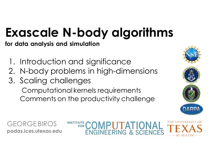
Exascale N-body algorithms for data analysis and simulation 1. - PowerPoint PPT Presentation

Exascale N-body algorithms for data analysis and simulation 1. Introduction and significance 2. N-body problems in high-dimensions 3. Scaling challenges Computational kernels requirements Comments on the productivity challenge GEORGE BIROS padas.ices.utexas.edu

With • Bill March • Bo Xiao • Chenhan Yu • Sameer Tharakan • Dhairya Malhotra

N-body methods O(N 2 ) à O(N) Gravity & Coulomb Waves & Scattering Fluids & Transport Machine learning Geostatistics Image analysis

MATVEC or Kernel sum

Relation to PDEs

Relation to H-matrices

Nystrom method (and its variants) • Most popular and effective method • Low-rank decomposition for the kernel matrix G (not an N-body algorithm) • Uses matrix sampling theory; requires random sampling of O(s) points, s is the target rank • Work • Error Talwalkar et al, 10

N-body 101

Idea I: Far-field interactions x x j x x x targets sources x w separation LOW RANK APPROXIMATION O(N 3 ) à O(N)

Idea II: Near-/Far-field split

Idea III: recursion 1 2 K 11 K 12 3 4 K 32 R d Matrix partitioning

Questions • Accurate far-field representation • Optimal complexity – N 2 à N log N à N • Error bounds • HPC – Parallelization – Good per/core performance – Heterogeneous architectures • For dim<4, all these are answered

Low dimensions • Barnes & Hut’86 – Treecodes • Greengard & Rokhlin’87 – FMM • Roklin’90 - High frequency FMM • Hackbusch & Novak’89 – Panel clustering • Hackbusch’99 – H-Matrices • Greengard & Gropp’91 – parallel • Warren & Salmon’93 - parallel

Stokes flow, 18B dof, jump =1E9 Malhotra, Gholami, B., SC’14 p: Stampede nodes node: 1.42TFLOP Xeon: 16 core ~ 22% peak

High-dimensions • Griebel et al’12: 200K points, synthetic 20D, real 6D, sequential • Duraiswami et al’06 (IFGT): 100K points, 9D, low-order accuracy, sequential • Tharakan, March, & B: 4.5M points, 28D, Nystrom • Lee, Vuduc & Gray: 20M points, 10D, low-order accuracy, parallel

Issues with high D • Approximation of far-field (polynomial in ambient-D) • • Pruning (near-far field) (polynomial in ambient-D) • • Practically, no scalable algorithms • no parallelism, no control of complexity/accuracy • Nystrom method assumes global low-rank doesn’t scale with problem size •

ASKIT SISC’15, SISC’16, ACHA’15, KDD’15, SC’15, IPDPS’15 • Far-field approximation—intrinsic D • Nearest Neighbors: Pruning/Sampling • Provable/predictable complexity estimate • Provable/predictable error estimate • Parallelism and performance • Inspired by: – Kapur & Long’98, Ying & B. & Zorin’03 – Halko & Martinsson & Tropp’11 Other related work ACA, CUR, Approximate QR –

Far-field approximation • G: n x m matrix ; compute factor(G) • Subsample G s , n s x m matrix factor(G s ) ~ factor(G) • uniform sampling (large errors) • norm sampling (better errors) • leverage sampling (close to optimal, requires SVD(G)) • range space sampling ( requires fast matvec(G) • ASKIT: random sampling + nearest neighbors • approximates norm sampling, behaves like leverage sampling – SKELETONIZATION –

Skeletonization : far field representation

Evaluation

Evaluation

Summary of ASKIT features • Metric tree to create binary partition • Approximate nearest-neighbors using RPTs • Nearest neighbors for skeletonization Far-field sampling to construct approximate ID • Pruning using tree Morton IDs • • Bottom-up pass to recursively create skeletons • Top-down pass, treecode evaluation • ID rank of far field is adaptively chosen give error tolerance (similar to FMM tolerance)

Theoretical results Work Error Nystrom

Gaussian kernel 3D, 1M points 64D, 8D intr, 1M points

8 M points / 784 dimensions March, B. et al KDD’15, SC’15 • OCR using multiclass kernel logistic regression

8M points, 784 dimensions NYSTROM ASKIT

Scaling March W, Yu C , B. et al, IPDPS 15 CLASSIFICATION 1B / 128D ~1TB TACC Stampede Largest run 144s 200 TFLOPS 30% peak

H-matrices and factorizations inverse

Scaling for INV-ASKIT IPDPS’16 N=0.5M, D=54 N=4.5M, D=8 For run #11 N=1.6M, D=784 we get 30 TFLOPS~ 35% peak N=16M, D=64

Toward exascale

Scalability requirements • Computational physics/chemistry/biology – large scale – 1E13 unknowns (3D/4D) Graphics/signal analysis • – real time – 1E6 unknowns (1D/4D) Data analysis/Uncertainty quantification • – large scale – 1E15 unknowns (1D - 1000D) – real time / streaming / online

Computational Kernels • Geometric – distance calculations / projections • Analytic – special functions / fast transforms / differentiation • Algebraic – QR factorization, Least squares • Combinatorial – tree traversals / pruning / sorting / merging • Statistical – sampling • Memory – reshuffling, packing, permutation, communication • Application – linear/non linear/optimization/time stepping / multiphysics

Kernel examples [problem size / node] Special function evaluations • Sorting/merging [1E5-1E9] • Median/selection [1-1E9] • Tree-traversals / neighborhood construction • Euclidean distance calculations [ GEMM-like 100—16,000 ) ] • Nearest-neighbors [ GEMM-like + heapsort ] • Kernel evaluations [ GEMM-like 100—16,000 ] • FFTs [3D, size./dim O(10)-O(20)] • High-order polynomial evaluations • Rectangular GEMM [ 8-500 X 100,000] • Pivoted QR factorizations [500 – 16,000] •

Nearest neighbor kernel x j x i

GEMM for nearest-neighbors • Input : O(Nd) • Output : O(N k) • Calculations: O(N 2 d + N k logk) • Intermediate storage: O(N 2 + Nk)

Custom GEMM + heap selection + arbitrary norms

Comparison with GEMM

The perspective of high- level application and library designers actually just my perspective - focus on single node only

Workflow Model selection Discretization - correctness and speed Verification Robustness / usability / reproducibility Validation PREDICT High performance and efficiency Our responsibility: develop algorithms that “respect” memory hierarchies, promote/expose SIMD, are work-optimal, concurrent, and fault tolerant

Our understanding of CPU • FLOPS = • MOPS – Cores x – Registers – FLOPS/instruction x – Cache – Instructions/cycle x – RAM – Cycles/sec – DISK • Try to block and vectorize

Code for correctness j C = A*B B k i k C A C

Example • C=A*B, all A,B,C 4000-by-4000 • 1 CORE Expected run time: 4000 3 * 2 / 21E9 = 6s • ICC -g : 80 s, 12X slower • ICC -O: 48 s 8X slower • ICC -O3: 25 s; 4X slower • 8 CORES: 3.4 s vs 0.75 (~4.5X slower) • 16 CORES: 2.6s vs 0.38 (~7X slower) • 16 CORES, gcc -O3: 60secs (~100X slower) • 2 x 8core-E5-2680 2.7GHz

Reality (BLIS) FLAME/BLIS van de Geijn group UT AUSTIN

Challenges for exascale • Large and constantly evolving design space • Expanding complexity of – simulation and data analysis – programming and profiling tools – underlying hardware • No common abstract parallel machine model • Static/synchronous scheduling increasingly hard • Fault tolerance / resiliency • End-to-end scalability

Gaps in programmability • Large percentage of productivity production scientific • codes ~ 1-0.1% efficiency maintenability • performance • Would be happy to have scalability • productivity tools that can raise performance to 10% portability • Requires 10X to 100X accessibility • improvements energy efficiency • reproducibility •

Thank you