Example - Newton-Raphson Method We now consider the following - PDF document

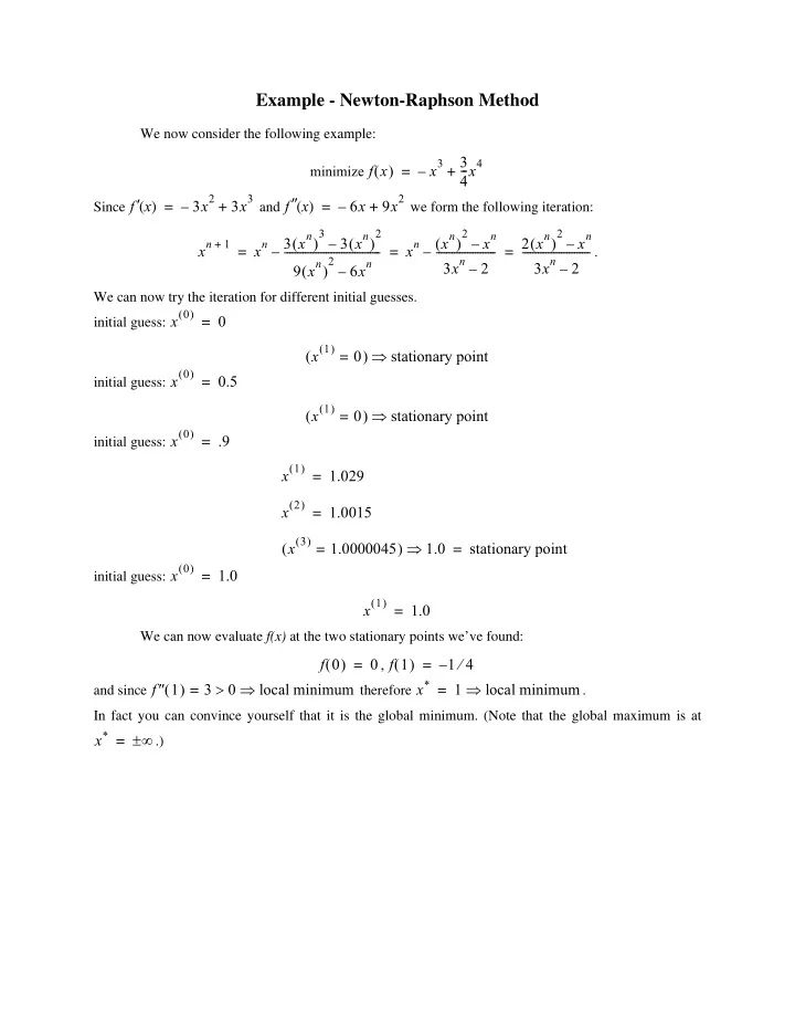
Example - Newton-Raphson Method We now consider the following example: 3 x 3 - x 4 ( ) - - f x = – + minimize 4 3 x 2 3 x 3 9 x 2 f ″ x f ′ x ( ) = – + ( ) = – 6 x + Since and we form the following iteration: 3 2 2 2 3 x n 3 x n x n x n 2 x n x n ( ) ( ) ( ) ( ) – – – x n + 1 x n x n = – - - - - - - - - - - - - - - - - - - - - - - - - - - - - - - - - - - - - - = – - - - - - - - - - - - - - - - - - - - - - - - = - - - - - - - - - - - - - - - - - - - - - - - - - - . 2 3 x n 3 x n 9 x n 6 x n – 2 – 2 ( ) – We can now try the iteration for different initial guesses. ( ) x 0 = 0 initial guess: ( ) x 1 ( ) ⇒ = 0 stationary point ( ) x 0 = 0.5 initial guess: ( ) x 1 ( ) ⇒ = 0 stationary point ( ) x 0 = .9 initial guess: ( ) x 1 = 1.029 ( ) x 2 = 1.0015 ( ) x 3 ( ) ⇒ = 1.0000045 1.0 = stationary point ( ) x 0 = initial guess: 1.0 ( ) x 1 = 1.0 We can now evaluate f(x) at the two stationary points we’ve found: ( ) ( ) ⁄ = = – f 0 0 f 1 1 4 , x * f ″ 1 ( ) > ⇒ ⇒ = 3 0 local minimum = 1 local minimum and since therefore . In fact you can convince yourself that it is the global minimum. (Note that the global maximum is at x * ± ∞ = .)

Interval Reduction Using Function Samples Only f 1 initial bracketed interval I 0 = [ a, b ] f 2 x a c d b ( ) < ( ) ⇒ f 1 : f 1 d f 1 c I 1 = [ , ] c b 1) consider , ( ) > ( ) ⇒ f 2 : f 2 d f 2 c I 1 = [ , ] a d 2) consider . x a x L x m x u b Algorithm: Interval Halving Search input a, b , ∆ min 1. // input the initial interval ∆ ∆ 2 ⁄ ( ) = b – a x m = a + f m = f x m 2. set: , , ∆ > ∆ min 3. while repeat ∆ 4 ⁄ ( ) x L = a + f L = f x L 4. set: , ∆ 4 ⁄ ( ) = – = 5. x u b , f u f x u < 6. if f L f m then ∆ b = x m x m = x L f m = f L = b – a 7. set , , , < f u f m 8. else if ∆ a = x m x m = x u f m = f u = b – a 9. set , , , 10. else ∆ a = x L b = x u = b – a 11. set , , 12. end if 13. end if 14. end while // final interval size is less than ∆ min 15. output [ a, b ] After 2 n+ 1 function evaluation the interval is reduced by ) n ( ⁄ 1 2 3 … , , I 2 n = I 0 1 2 n = , + 1 I o where is the size of the initial interval.

Fibonacci Search Technique Question How should we pick N successive points in an interval to perform function evaluations ( ) f x such that the final reduced interval is the smallest possible irrespective of the properties of ? initial interval: [0, 2] new interval: [0, 1+ δ ] x 1 1+ δ 0 2 Best location for two function evaluations N = 3 initial interval: [0, 3] final interval: [1, 2] x 1 1+ δ 0 2 3 N = 4 initial interval: [0, 5] final interval: [4, 5] x 4+ δ 0 1 2 3 4 5 N = 5 initial interval: [0, 8] final interval: [4, 5] x 1+ δ 0 1 2 3 4 5 8 Examples of optimal sampling locations Fibonacci sequence of numbers: ( )∞ F 0 = F 1 = 1 F i = F i + F i i = 2 1 , , . – 1 – 2 , F i F i F i Given an interval of proportion and choosing two sample points at . – 2 – 1

initial interval: [0, F i ] new interval: [0, F i-1 ] or [ F i-2 , F i ] x 0 F i-2 F i-1 F i Fibonacci type sampling The new interval will be either [ , 0 F i ] [ F i , F i ] or – – 1 2 F i F i – F i = F i the first has size , the second has size and therefore they are the same size. The – 1 – 2 – 1 F i F i – F i next point is chosen as either or . – 3 – 3 ⁄ ⁄ I N I 0 = 1 F N The interval reduction is equal to after N function evaluations. It has been shown that this is the best possible reduction for a given number of function evaluations. At each step the ⁄ F i F i F N reduction is equal to . The drawback of this procedure is that you must start with and work + 1 backwards down the sequence. Golden Section Search [ , ] 0 1 x 1 and x 2 Given a normalized interval where should two points be chosen such that: 1) size of reduced interval is independent of function. 2) only one function evaluation per interval reduction. if f 2 < f 1 then new interval is [0, x 1 ] 0 x 2 x 1 1 if f 1 < f 2 then new interval is [ x 2 , 1] 0 x 2 x 1 1 Golden section interval reduction, initial interval is [0, 1].

Therefore by condition 1 above x 1 – 0 = 1 – x 2 x 2 = 1 – x 1 or and by condition 2 – – x 1 x 2 1 x 1 - - - - - - - - - - - - - - - - = - - - - - - - - - - - - - - x 1 1 2 2 ⇒ – = – = x 1 x 2 x 1 x 1 x 1 x 2 from 2 ⇒ τ x 1 + x 1 – 1 = 0 x 1 = = .61803 τ 2 θ τ x 2 = 1 – x 1 = .38197 = = 1 – = τ θ where we call the golden section and the golden mean. θ τ After each function evaluation and comparison of the interval is eliminated or of the original interval remains. Thus after N function evaluations an interval of original size L will be reduced to a size L τ N – 1 Algorithm: Golden Section search 1. input a 1 , b 1 , tol ( τ ) b 1 ( ) , F c ( ) = + – – = 2. set c 1 a 1 1 a 1 F c 1 ( τ ) b 1 ( ) , F d ( ) d 1 = b 1 – 1 – – a 1 = F d 1 3. 1 2 … repeat , , K = 4. for < F c F d 5. if then , , a k = a k b k = d k d k = c k 6. set + 1 + 1 + 1 ( τ ) ( ) c k = a k + 1 – b k – a k 7. + 1 + 1 + 1 + 1 , ( ) F d = F c F c = F c k 8. + 1 9. else , , = = = 10. set a k c k b k b k c k d k + 1 + 1 + 1 ( τ ) ( ) = – – – 11. d k b k 1 b k a k + 1 + 1 + 1 + 1 , ( ) F c = F d F d = F d k 12. + 1 13. end < b k – a k tol 14. end until + + 1 1 < interval tol Notes: iterate until

Polynomial Interpolation Methods In an interval of uncertainty the function is approximated by a polynomial and the minimum of the polynomial is used to predict the minimum of the function. Quadratic Interpolation px 2 ( ) F x = + qx + r If is the interpolating quadratic we need to find the coefficients p , q , and r < < ( ) ( ) [ , ] = = given the end points of the interval a b and c such that a c b with F a F a F b F b , ( ) F c = F c . The coefficients satisfy the matrix equation a 2 a 1 F a p b 2 b 1 = F b q c 2 c 1 r F c which can be easily solved analytically. Once we have the coefficients we need to find the minimum of F(x) and thus d F x ( ) ( ) = g x * = 2 px * + q = 0 d x q x * = – - - - - - - 2 p and therefore we only need the q and p coefficients. These can be solved using Cramer’s rule: F a a 1 ( ) ( ) ( ) F a b – c + F b c – a + F c a – b 1 - - - p = = - - - - - - - - - - - - - - - - - - - - - - - - - - - - - - - - - - - - - - - - - - - - - - - - - - - - - - - - - - - - - - - - - - - - - - - - - - - - - - - - - F b b 1 ∆ ∆ F c c 1 a 2 F a 1 F a b 2 c 2 F b a 2 c 2 F c a 2 b 2 ( ) ( ) ( ) – + – – – 1 b 2 F b 1 - - - q = = – - - - - - - - - - - - - - - - - - - - - - - - - - - - - - - - - - - - - - - - - - - - - - - - - - - - - - - - - - - - - - - - - - - - - - - - - - - - - - - - - - - - - - - - - - - - - - - - - ∆ ∆ c 2 F c 1 and therefore - F a b 2 c 2 F b c 2 a 2 F c a 2 b 2 ( ) ( ) ( ) – + – + – 1 q - - - - - - - - - - - - - - - - - - - - - - - - - - - - - - - - - - - - - - - - - - - - - - - - - - - - - - - - - - - - - - - - - - - - - - - - - - - - - - - - - - - - - - - - - - - - - - - - - - x * = – - - - - - - = ( ) ( ) ( ) 2 F a b – c + F b c – a + F c a – b 2 p

⇐ x * [ , ] a b Notice that must lie in if F c < F a and F c < F b bracketing interval. Also note that f ″ x * ( ) ( ) ( ) > 0 ⇒ = 2 p x * p x * and therefore if local minimum of quadratic whereas if ( ) < 0 ⇒ p x * local maximum. f x * ( ) ( ) We now evaluate and compare it to f c in order to reduce the interval of uncertainty. f(x) f(x*) > f c k a k x* c k b k x a k+1 c k+1 b k+1 ⇒ f(x*) > f c k new interval is [ a k+1 , b k+1 ] and new c value is c k+1 f(x) f(x*) < f c k a k x* c k b k x a k+1 c k+1 b k+1 ⇒ f(x*) < f c k new interval is [ a k+1 , b k+1 ] and new c value is c k+1