Exact Camera Location Recovery by Least Unsquared Deviations Gilad - PowerPoint PPT Presentation

Exact Camera Location Recovery by Least Unsquared Deviations Gilad Lerman University of Minnesota Joint work with Yunpeng Shi (University of Minnesota) and Teng Zhang (University of Central Florida) Gilad Lerman 1 / 23

Content 1 Introduction Structure from motion Camera location recovery 2 Previous Works 3 New theoretical guarantees 4 Conclusion Gilad Lerman 2 / 23

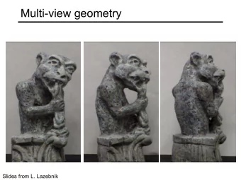
Structure from motion (SfM) ❼ Input: 2D images of the same object from different views ❼ Output: 3D structure of the object Demonstration by Snavely et al. (2006) Gilad Lerman 3 / 23

Pipeline of Structure from Motion ❼ Keypoint matching ❼ Essential matrix estimation ❼ Camera orientation estimation ❼ Camera location estimation Gilad Lerman 4 / 23

❼ ❼ ❼ ❼ Camera Location Recovery ❼ Input: Possibly corrupted pairwise directions between some cameras ❼ Output: Camera locations Gilad Lerman 5 / 23

❼ ❼ ❼ Camera Location Recovery ❼ Input: Possibly corrupted pairwise directions between some cameras ❼ Output: Camera locations ❼ Example: Recovery of 4 locations from 5 uncorrupted pairwise directions Gilad Lerman 5 / 23

❼ ❼ Camera Location Recovery ❼ Input: Possibly corrupted pairwise directions between some cameras ❼ Output: Camera locations ❼ Example: Recovery of 4 locations from 5 uncorrupted pairwise directions ❼ The problem is defined up to shift and scale Gilad Lerman 5 / 23

Camera Location Recovery ❼ Input: Possibly corrupted pairwise directions between some cameras ❼ Output: Camera locations ❼ Example: Recovery of 4 locations from 5 uncorrupted pairwise directions ❼ The problem is defined up to shift and scale ❼ Unique solution (up to shift and scale) may not exist ❼ Graphs whose vertex locations are recoverable from edge directions are called Parallel Rigid Gilad Lerman 5 / 23

❼ Example of non-parallel rigid graphs: Gilad Lerman 6 / 23

❼ Generative Graph Model for Camera Location Recovery ❼ The HLV model is due to Hand, Lee and Voroniski (2015) ❼ It has parameters n ∈ N , 0 ≤ p ≤ 1 and 0 ≤ ǫ b ≤ 1 Gilad Lerman 7 / 23

Generative Graph Model for Camera Location Recovery ❼ The HLV model is due to Hand, Lee and Voroniski (2015) ❼ It has parameters n ∈ N , 0 ≤ p ≤ 1 and 0 ≤ ǫ b ≤ 1 ❼ Step 1 : Generate the following graph with vertices V ∶ = { t ∗ i } n i = 1 ⊆ R 3 i.i.d. ∼ N ( 0 , I ) Gilad Lerman 7 / 23

Generative Graph Model for Camera Location Recovery ❼ Step 2 : The set of edges E are drawn i.i.d. from { ij ∶ 1 ≤ i ≠ j ≤ n } with probability p (Erd¨ os-R´ enyi graph) Gilad Lerman 8 / 23

Generative Graph Model for Camera Location Recovery ❼ Step 3 : For each ij ∈ E , assign the true pairwise direction t ∗ i − t ∗ j γ ij = γ ∗ ij ∶ = ∥ t ∗ i − t ∗ j ∥ Gilad Lerman 9 / 23

Generative Graph Model for Camera Location Recovery ❼ Step 4 : Corrupt the generated graph ▸ Pick a subgraph G b ( V,E b ) such that E b ⊆ E and the maximal degree of G b < ǫ b n . The set of uncorrupted edges is E g ∶ = E ∖ E b ▸ For all ij ∈ E b , replace γ ij by arbitrary unit vector Gilad Lerman 10 / 23

Generative Graph Model for Camera Location Recovery ❼ (Optional) Step 5 : Add the noise γ ij + σ v ij ▸ For all ij ∈ E g , let γ ij = ∥ γ ij + σ v ij ∥ , where σ > 0 is noise level and v ij iid ∼ N ( 0 , I ) Gilad Lerman 11 / 23

Least Squares Camera Location Solvers ❼ Least Squares Solver (M. Brand and et al., 2004): ⎧ i = 1 ∥ t i ∥ 2 = 1 ⎪ ∑ n ⎪ ij ( t i − t j )∥ 2 s.t. ∥ P γ ⊥ ⎨ i = 1 ⊂ R 3 ∑ min , ⎪ ∑ n i = 1 t i = 0 ⎪ { t i } n ⎩ ij ∈ E where P γ ⊥ ij denotes the orthogonal projection onto the orthogonal complement of γ ij ❼ Constrained Least Squares Solver (Tron and Vidal, 2009): ⎧ ⎪ α ij ≥ 1 ⎪ ∥ t i − t j − α ij γ ij ∥ 2 s.t. ⎨ ∑ min ⎪ ∑ n i = 1 t i = 0 ⎪ { t i } n i = 1 ⊂ R 3 ⎩ ij ∈ E { αij } ij ∈ E ⊂ R Gilad Lerman 12 / 23

Current Robust Location Solvers ❼ LUD: Least Unsquared Deviations (Ozyesil and Singer, 2015): ⎧ ⎪ ⎪ α ij ≥ 1 ∥ t i − t j − α ij γ ij ∥ s.t. ⎨ ∑ min ⎪ ∑ n i = 1 t i = 0 ⎪ { t i } n i = 1 ⊂ R 3 ⎩ ij ∈ E { αij } ij ∈ E ⊂ R ❼ ShapeFit (Hand, Lee and Voroninski, 2015): ⎧ ⎪ ⎪ ∑ ij ∈ E ⟨ t i − t j , γ ij ⟩ = 1 ∥ P γ ⊥ ij ( t i − t j )∥ s.t. ⎨ i = 1 ⊂ R 3 ∑ min , ⎪ ∑ n i = 1 t i = 0 ⎪ { t i } n ⎩ ij ∈ E where P γ ⊥ ij denotes the orthogonal projection onto the orthogonal complement of γ ij Gilad Lerman 13 / 23

Empirical performance of LUD and ShapeFit ❼ Performance of LUD and ShapeFit for synthetic data with corruption and noise Gilad Lerman 14 / 23

Theoretical Guarantees Theorem 0 (Hand, Lee and Voroninski, 2015) There exist absolute constants n 0 , C 0 and C 1 such that for n > n 0 and for i = 1 ⊆ R 3 , E ⊆ [ n ] × [ n ] and { γ ij } ij ∈ E ⊆ R 3 generated by the HLV { t ∗ i } n model with parameters n , p and ǫ b satisfying C 0 n − 1 / 5 log 3 / 5 n ≤ p ≤ 1 and ǫ b ≤ C 1 p 5 / log 3 n , ShapeFit recovers { t ∗ i } n i = 1 up to shift and scale with probability 1 − 1 / n 4 . Gilad Lerman 15 / 23

Theoretical Guarantees Theorem 0 (Hand, Lee and Voroninski, 2015) There exist absolute constants n 0 , C 0 and C 1 such that for n > n 0 and for i = 1 ⊆ R 3 , E ⊆ [ n ] × [ n ] and { γ ij } ij ∈ E ⊆ R 3 generated by the HLV { t ∗ i } n model with parameters n , p and ǫ b satisfying C 0 n − 1 / 5 log 3 / 5 n ≤ p ≤ 1 and ǫ b ≤ C 1 p 5 / log 3 n , ShapeFit recovers { t ∗ i } n i = 1 up to shift and scale with probability 1 − 1 / n 4 . Theorem 1 (L, Shi and Zhang, 2017) There exist absolute constants n 0 , C 0 and C 1 such that for n > n 0 and for i = 1 ⊆ R 3 , E ⊆ [ n ] × [ n ] and { γ ij } ij ∈ E ⊆ R 3 generated by the HLV { t ∗ i } n model with parameters n , p and ǫ b satisfying C 0 n − 1 / 3 log 1 / 3 n ≤ p ≤ 1 and ǫ b ≤ C 1 p 7 / 3 / log 9 / 2 n , LUD recovers { t ∗ i } n i = 1 up to shift and scale with probability 1 − 1 / n 4 . Gilad Lerman 15 / 23

Part1 of Proof: Reformulation of LUD ❼ Recall LUD: ⎧ ⎪ α ij ≥ 1 ⎪ t i } n ({ ˆ i = 1 , { ˆ α ij } ij ∈ E ) = arg min ∑ ∥ t i − t j − α ij γ ij ∥ s.t. ⎨ ⎪ ∑ i t i = 0 ⎪ { t i } n i = 1 ⊂ R 3 ⎩ ij ∈ E { αij } ij ∈ E ⊂ R ❼ Expression for ˆ α ij in two complementary cases: Case 2: ⟨ ˆ t i − ˆ t j , γ ij ⟩ ≤ 1 Case 1: ⟨ ˆ t i − ˆ t j , γ ij ⟩ > 1 ˆ t i − ˆ t i − ˆ ˆ t j t j γ ij = ˆ γ ij 0 α ij γ ij ˆ 0 α ij γ ij α ij = ⟨ ˆ t i − ˆ t j , γ ij ⟩ α ij = 1 Here ˆ Here ˆ Gilad Lerman 16 / 23

Reformulation of LUD ❼ Recall LUD: ⎧ ⎪ α ij ≥ 1 ⎪ ({ ˆ t i } n i = 1 , { ˆ α ij } ij ∈ E ) = arg min ∥ t i − t j − α ij γ ij ∥ s.t. ⎨ ∑ ⎪ ∑ i t i = 0 ⎪ { t i } n i = 1 ⊂ R 3 ⎩ ij ∈ E { αij } ij ∈ E ⊂ R ❼ Expression for ˆ α ij : ⎧ ⎪ ⎪ ⟨ ˆ t i − ˆ t j , γ ij ⟩ , if ⟨ ˆ t i − ˆ t j , γ ij ⟩ > 1; α ij = ⎨ ˆ ⎪ if ⟨ ˆ t i − ˆ t j , γ ij ⟩ ≤ 1 ⎪ 1 , ⎩ ❼ Reformulation: { ˆ t i } n i = 1 = f ij ( t i , t j ) subject to ∑ n i = 1 t i = 0 , i = 1 ⊂ R 3 ∑ min { t i } n ij ∈ E ⎧ ⎪ ∥ P γ ⊥ ij ( t i − t j )∥ , if ⟨ t i − t j , γ ij ⟩ > 1; ⎪ where f ij ( t i , t j ) = ⎨ ⎪ ⎪ ∥ t i − t j − γ ij ∥ , if ⟨ t i − t j , γ ij ⟩ ≤ 1 ⎩ Gilad Lerman 17 / 23

Part 2 of the Proof: Optimality Condition ❼ WLOG, assume that { t ∗ i } n i = 1 is already centered at 0 ❼ Goal : Show that under a certain condition any perturbation from the ground truth { c ∗ t ∗ i } n i = 1 increases the value of the objective function, where c ∗ = arg min f ij ( c t ∗ i ,c t ∗ j ) ∑ c ∈ R ij ∈ E Gilad Lerman 18 / 23

Adaptation of ShapeFit Analysis ❼ Observation: On long edges, i.e., ∥ t ∗ i − t ∗ j ∥ > 1 c ∗ , the objective functions of ShapeFit and LUD coincide for the ground truth solution { ˆ t i } n i = 1 = { c ∗ t ∗ i } n i = 1 ❼ Define the set of good and long edges, E gl = { ij ∈ E g ∣ ∥ t ∗ i − t ∗ j ∥ > 1 / c ∗ } , and its complement E c gl = E ∖ E gl ❼ The analysis of ShapeFit with E g and E c g is replaced with E gl and E c gl Gilad Lerman 19 / 23

Good-Long-Dominance Condition Definition 1 V = { t ∗ i } n i = 1 , E ⊆ [ n ] × [ n ] and { γ ij } ij ∈ E satisfy the good-long-dominance i = 1 ∈ R 3 such that ∑ n condition if for any perturbation vectors { ǫ i } n i = 1 ǫ i = 0 and ∑ n i = 1 ⟨ ǫ i , t ∗ i ⟩ = 0 , ∥ P γ ∗⊥ ij ( ǫ i − ǫ j )∥ ≥ ∑ ∥ ǫ i − ǫ j ∥ . ∑ ij ∈ E c ij ∈ E gl gl Theorem 2 If V = { t ∗ i } n i = 1 , E ⊆ [ n ] × [ n ] and { γ ij } ij ∈ E satisfy the good-long-dominance condition, then LUD exactly recovers the ground truth solution up to shift and scale. Gilad Lerman 20 / 23