Evaluating Estimators Statistical evaluation ways of choosing with- - PowerPoint PPT Presentation

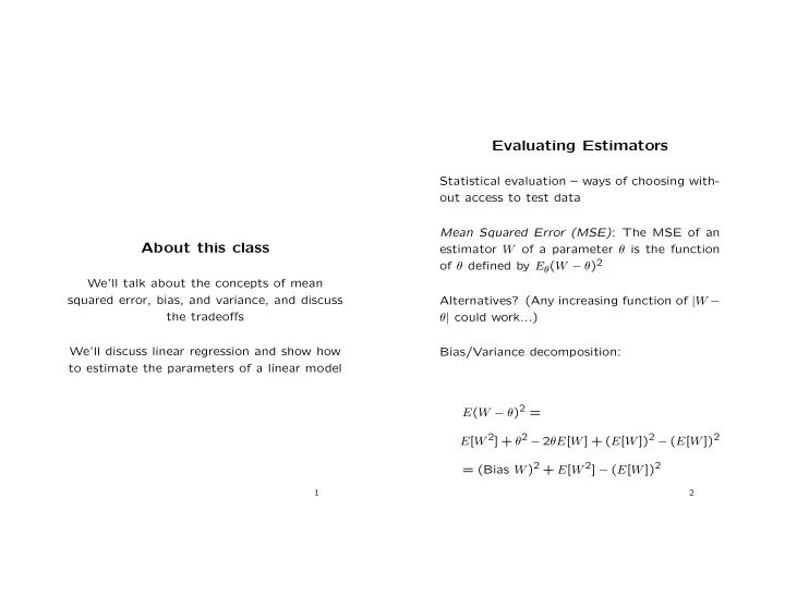
Evaluating Estimators Statistical evaluation – ways of choosing with- out access to test data Mean Squared Error (MSE) : The MSE of an About this class estimator W of a parameter θ is the function of θ defined by E θ ( W − θ ) 2 We’ll talk about the concepts of mean squared error, bias, and variance, and discuss Alternatives? (Any increasing function of | W − the tradeo ff s θ | could work...) We’ll discuss linear regression and show how Bias/Variance decomposition: to estimate the parameters of a linear model E ( W − θ ) 2 = E [ W 2 ] + θ 2 − 2 θ E [ W ] + ( E [ W ]) 2 − ( E [ W ]) 2 = (Bias W ) 2 + E [ W 2 ] − ( E [ W ]) 2 1 2

Estimators for the Normal Distribution Let X 1 , . . . , X n be iid N ( µ, σ 2 ) Unbiased estimator for mean is sample mean = (Var W ) + (Bias W ) 2 Unbiased estimator for variance is the sample variance: where n 1 S 2 = ( X i − X ) 2 � Bias W = E θ W − θ n − 1 i =1 Proof: Unbiased estimators ( E θ W = θ for all θ ) are n 1 good at controlling bias! An unbiased estima- E [ S 2 ] = E [ ( X i − X ) 2 ) � n − 1( tor has MSE equal to its variance i =1 n n 1 i ) + nX 2 − 2 X X 2 � � = n − 1[ E ( X i ] i =1 i =1 n 1 i − nX 2 ) X 2 � = n − 1 E ( i =1 3

1 Proof: 1 − nEX 2 ) n − 1( nEX 2 = n n n g ( X i ))] 2 � � � Var g ( X i ) = E [ g ( X i ) − E ( i =1 i =1 i =1 Now we need to use a couple of additional n facts: ( g ( X i ) − Eg ( X i ))] 2 � = E [ i =1 1 − ( EX 1 ) 2 = σ 2 If we expand this, there are n terms of the form EX 2 ( g ( X i ) − Eg ( X i )) 2 and EX 2 − ( EX ) 2 = σ 2 /n The expectation of this term is Var g ( X i ). There- fore, for n of them we get n Var g ( X 1 ). (This second is basically the definition of stan- dard error) What about the other terms? They are all of the form: To show the second, here’s a lemma: ( g ( X i ) − Eg ( X i ))( g ( X j ) − Eg ( X j )) n � Var g ( X i ) = n Var g ( X 1 ) with i � = j The expectation of this is the co- i =1 variance of X i and X j , which is 0 from inde- (where Eg ( X i )) and Var g ( X i ) exist) pendence.

MSEs for Estimators for the Normal Distribution Unbiased estimator for the mean µ is X Unbi- ased estimator for the variance σ 2 is S 2 MSEs for these estimators are: Now we plug back into the expression for E [ S 2 ] E ( X − µ ) 2 = Var X = σ 2 and find: n 1 1 − nEX 2 ) E [ S 2 ] = n − 1( nEX 2 E ( S 2 − σ 2 ) 2 = Var S 2 = 2 σ 4 n − 1 n − 1( n ( σ 2 + µ 2 ) − n ( σ 2 1 n + µ 2 )) = σ 2 = 1 � n MLE for the variance is ˆ i =1 ( X i − n X ) 2 = n − 1 n S 2 = σ 2 σ 2 = E ( n − 1 S 2 ) = ( n − 1 ) σ 2 E ˆ n n σ 2 = Var ( n − 1 S 2 ) Var ˆ n 4

= ( n − 1 ) 2 Var S 2 n Bias/Variance Tradeo ff in General ) 2 2 σ 4 = ( n − 1 Keep in mind: MSE is not the last word. Should n n − 1 we be comfortable using biased estimators? = 2( n − 1) σ 4 Why are they biased? n 2 Is MSE reasonable for scale parameters (as op- MSE, using the bias/variance decomposition posed to location ones?) – forgives underesti- σ 2 − σ 2 ) 2 = 2( n − 1) σ 4 + ( n − 1 mation... σ 2 − σ 2 ) 2 E (ˆ n 2 n Hypothesis space too simple? High bias, low = 2 n − 1 σ 4 variance n 2 Which is less than Hypothesis space too complex? Low bias, high 2 σ 4 variance n − 1 5

Least Squares Regression Define x and y as usual from our sample data. Statistics: describing data, inferring conclu- Now define: sions n ( x i − x ) 2 � S xx = Machine learning: predicting future data (out- i =1 of-sample) n ( y i − y ) 2 � S yy = What would be a reasonable thing to do in the i =1 following case (diagram of point cloud)? n � S xy = ( x i − x )( y i − y ) i =1 Assumption for linear regression: data can be modeled by Let’s fit a line to the data as best as we can. y i = α + β x i + ǫ i How do we define this? Residual sum of squares (RSS) n First algorithmic question for us: how to find ( y i − ( c + dx i )) 2 � α and β ? i =1 6 7

n n n Now, find a and b , estimators of α and β , such ( x i − x ) 2 +2 ( x − a ) 2 � � � = ( x i − x )( x − a )+ that: i =1 i =1 i =1 n n Second term drops out, basically giving us our ( y i − ( c + dx i )) 2 = ( y i − ( a + bx i )) 2 � � min result c,d i =1 i =1 For a given value of d , the minimum value of For any fixed value of d , the minimizing value RSS is then of c can be found as follows. n n n (( y i − dx i ) − ( y − dx )) 2 ( y i − ( c + dx i )) 2 = (( y i − dx i ) − c ) 2 � � � i =1 i =1 i =1 n (( y i − y ) − d ( x i − x )) 2 � = Turns out the right side is minimized at i =1 n c = 1 � ( y i − dx i ) = S yy − 2 dS xy + d 2 S xx n i =1 Take the derivative with respect to d and set = y − dx to 0 − 2 S xy + 2 dS xx = 0 Why? n n ⇒ d = S xy ( x i − a ) 2 = min ( x i − x + x − a ) 2 � � min S xx a a i =1 i =1

A Statistical Method: BLUE Assumptions: EY i = α + β x i Var Y i = σ 2 Second one implies that variance is the same for all data points No assumption needed on the distribution of the Y i We’ll get di ff erent lines if we regress x on y ! (exercise) BLUE: Best Linear Unbiased Estimator Linear: estimator of the form � n i =1 d i Y i Unbiased: estimator must satisfy E � n i =1 d i Y i = β Therefore β = � n i =1 d i E [ Y i ] n � = d i ( α + β x i ) i =1 8

n n � � = α d i + β d i x i i =1 i =1 Must hold for all α and β . This is true i ff � n i =1 d i = 0 and � n i =1 d i x i = 1 The advantage of working under statistically Best: Smallest variance (Equal to MSE for un- explicit assumptions is we also get statistical biased estimators) knowledge about our estimator n n n i = σ 2 d 2 � � Var b = σ 2 d 2 Var d i Y i = i Var Y i � S xx i =1 i =1 i =1 n n i σ 2 = σ 2 d 2 d 2 � � = If you can choose the x i , you can design the i i =1 i =1 experiment to try and minimize the variance! The BLUE is then defined by constants d i that Similar analysis shows that the BLUE of α is minimize � n i =1 d 2 i while satisfying the constraints the same a as in least squares derived above. It turns out that the choices d i = x i − x S xx are the choices that do this, which gives us b = S xy S xx