Euler hydrodynamics for attractive particle systems in random - PowerPoint PPT Presentation

The model and its construction Hydrodynamic The disorder-particle process Other Models Euler hydrodynamics for attractive particle systems in random environment C. Bahadoran 1 , H. Guiol 2 , K. Ravishankar 3 & E. Saada 4 1 Universit´ e Clermont-Ferrand - France 2 Grenoble Universit´ es - France 3 SUNY College at New Paltz - USA 4 CNRS, Paris Descartes - France Condensation in Stochastic Particle Systems, Warwick, January 8, 2013

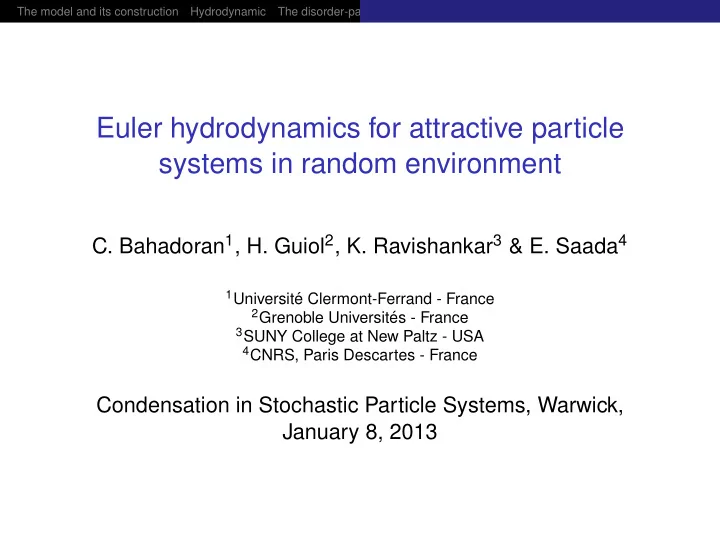
The model and its construction Hydrodynamic The disorder-particle process Other Models Outline The model and its construction Basic example : The ASEP (without disorder) The Misanthrope type model (without disorder) The model in random environment Hydrodynamic result Hydrodynamic theorem Flux function Previous results The disorder-particle process Other Models Generalized misanthropes’ process Generalized k -step K -exclusion process

The model and its construction Hydrodynamic The disorder-particle process ASEP The model Other Models The model in RE Basic example : The ASEP (without disorder) � � � � � � � � � � � � � � � � � � � � � � � � x y ◮ K = 1, for z ∈ Z , η ( z ) = 0 or 1. ◮ From each site x , choice of y with p ( y − x ) . ◮ According to (independent) exponential clocks, jump from x to y if possible ( exclusion rule ).

The model and its construction Hydrodynamic The disorder-particle process ASEP The model Other Models The model in RE Graphical construction [Harris] P = I P 0 × I P H for initial configurations and Poisson processes. I (below for ASEP) � basic coupling. t p q x x-1 x+1 x+2

The model and its construction Hydrodynamic The disorder-particle process ASEP The model Other Models The model in RE Graphical construction [Harris] P = I P 0 × I P H for initial configurations and Poisson processes. I (below for ASEP) � basic coupling. t p q x x-1 x+1 x+2

The model and its construction Hydrodynamic The disorder-particle process ASEP The model Other Models The model in RE Graphical construction [Harris] P = I P 0 × I P H for initial configurations and Poisson processes. I (below for ASEP) � basic coupling. t p q x x-1 x+1 x+2

The model and its construction Hydrodynamic The disorder-particle process ASEP The model Other Models The model in RE Graphical construction [Harris] P = I P 0 × I P H for initial configurations and Poisson processes. I (below for ASEP) � basic coupling. t p q x x-1 x+1 x+2

The model and its construction Hydrodynamic The disorder-particle process ASEP The model Other Models The model in RE Graphical construction [Harris] P = I P 0 × I P H for initial configurations and Poisson processes. I (below for ASEP) � basic coupling. t p q x x-1 x+1 x+2

The model and its construction Hydrodynamic The disorder-particle process ASEP The model Other Models The model in RE Graphical construction [Harris] P = I P 0 × I P H for initial configurations and Poisson processes. I (below for ASEP) � basic coupling. t p q x x-1 x+1 x+2

The model and its construction Hydrodynamic The disorder-particle process ASEP The model Other Models The model in RE Graphical construction [Harris] P = I P 0 × I P H for initial configurations and Poisson processes. I (below for ASEP) � basic coupling. t p q x x-1 x+1 x+2

The model and its construction Hydrodynamic The disorder-particle process ASEP The model Other Models The model in RE Graphical construction [Harris] P = I P 0 × I P H for initial configurations and Poisson processes. I (below for ASEP) � basic coupling. t p q x x-1 x+1 x+2

The model and its construction Hydrodynamic The disorder-particle process ASEP The model Other Models The model in RE Graphical construction [Harris] P = I P 0 × I P H for initial configurations and Poisson processes. I (below for ASEP) � basic coupling. t p q x x-1 x+1 x+2

The model and its construction Hydrodynamic The disorder-particle process ASEP The model Other Models The model in RE Graphical construction [Harris] P = I P 0 × I P H for initial configurations and Poisson processes. I (below for ASEP) � basic coupling. t p q x x-1 x+1 x+2

The model and its construction Hydrodynamic The disorder-particle process ASEP The model Other Models The model in RE Attractive Systems The Markov process ( η t ) t ≥ 0 with generator L and semigroup S ( t ) is attractive : ◮ partial order on X : η ≤ ξ ⇔ ∀ x ∈ Z , η ( x ) ≤ ξ ( x ) . Extended to probabilities on X : µ 1 ≤ µ 2 ◮ basic coupling : ( η t , ξ t ) t ≥ 0 on X × X ; η t and ξ t obey the same clocks. η 0 ≤ ξ 0 a.s. ⇒ η t ≤ ξ t a.s. ∀ t > 0.

The model and its construction Hydrodynamic The disorder-particle process ASEP The model Other Models The model in RE The Misanthrope type model (without disorder) State space X = { 0 , · · · , K } Z , η ∈ X , 0 ≤ η ( x ) ≤ K , ∀ x ∈ Z � p ( y − x ) b ( η ( x ) , η ( y )) [ f ( η x , y ) − f ( η )] Lf ( η ) = x , y ∈ Z ◮ (A1) Irreducibility : ∀ z ∈ Z , � n ∈ N [ p ∗ n ( z ) + p ∗ n ( − z )] > 0 ; ◮ (A2) finite mean : � z ∈ Z | z | p ( z ) < + ∞ ; ◮ (A3) K -exclusion rule : b ( 0 , . ) = 0 , b ( ., K ) = 0 ; ◮ (A4) non-degeneracy : b ( 1 , K − 1 ) > 0 ; ◮ (A5) attractiveness : b ( i , j ) nondecreasing in i , nonincreasing in j . Some Classical Examples : ◮ Simple Exclusion : K = 1, b ( 1 , 0 ) = 1 [Liggett] ◮ T.A. K -exclusion : p ( 1 ) = 1, b ( i , j ) = I { i > 0 , j < K } [Sepp¨ al¨ ainen] ◮ Misanthropes : + algebraic relations on b ’s [Cocozza]

The model and its construction Hydrodynamic The disorder-particle process ASEP The model Other Models The model in RE The model in random environment Disorder α = ( α ( x ) , x ∈ Z ) ∈ A = ( c , 1 / c ) Z , for c ∈ ( 0 , 1 ) . The dist. Q of α on A is ergodic w.r.t. τ x (on Z ). For α ∈ A , quenched process ( η t ) t ≥ 0 on X = { 0 , · · · , K } Z : � α ( x ) p ( y − x ) b ( η ( x ) , η ( y )) [ f ( η x , y ) − f ( η )] L α f ( η ) = (1) x , y ∈ Z Our method is robust w.r.t. the model and disorder (e.g. no restriction to site or bond disorder). We detail the misanthropes’ process with site disorder, then explain how to deal with other models.

The model and its construction Hydrodynamic The disorder-particle process ASEP The model Other Models The model in RE Graphical construction Let V = Z × [ 0 , 1 ] , (Ω , F , I P ) proba. space of locally finite point measures ω ( dt , dx , dv ) on R + × Z × V , where F is generated by the mappings ω �→ ω ( S ) for Borel sets S of R + × Z × V , and P makes ω a Poisson process with intensity I M ( dt , dx , dv ) = λ R + ( dt ) λ Z ( dx ) m ( dv ) where λ denotes either the Lebesgue or the counting measure. I E denotes expectation with respect to I P . For the case (1) we take V := Z × [ 0 , 1 ] , v = ( z , u ) ∈ V , m ( dv ) = c − 1 || b || ∞ p ( dz ) λ [ 0 , 1 ] ( du ) (2)

The model and its construction Hydrodynamic The disorder-particle process ASEP The model Other Models The model in RE (A2) ⇒ for I P -a.e. ω , ∃ a unique mapping ( α, η 0 , t ) ∈ A × X × R + �→ η t = η t ( α, η 0 , ω ) ∈ X (3) satisfying : (a) t �→ η t ( α, η 0 , ω ) is right-continuous ; (b) η 0 ( α, η 0 , ω ) = η 0 ; (c) the particle configuration is updated at points ( t , x , v ) ∈ ω (and only at such points - where ( t , x , v ) ∈ ω means ω { ( t , x , v ) } = 1) according to the rule η t ( α, η 0 , ω ) = T α, x , v η t − ( α, η 0 , ω ) (4) where, for v = ( z , u ) ∈ V ,  u < α ( x ) b ( η ( x ) , η ( x + z ))  η x , x + z if T α, x , v η = c − 1 || b || ∞ (5)  η otherwise Shift commutation property T τ x α, y , v τ x = τ x T α, y + x , v (6) where τ x on the r.h.s. acts only on η .

The model and its construction Hydrodynamic The disorder-particle process ASEP The model Other Models The model in RE Attractiveness By (A5) , T α, x , v : X → X is nondecreasing (7) Hence, ( α, η 0 , t ) �→ η t ( α, η 0 , ω ) is nondecreasing w.r.t. η 0 (8) Thus for any t ∈ R + and continuous function f on X , E [ f ( η t ( α, η 0 , ω ))] = S α ( t ) f ( η 0 ) , where S α denotes the I semigroup generated by L α . From (8), for µ 1 , µ 2 ∈ P ( X ) , µ 1 ≤ µ 2 ⇒ ∀ t ∈ R + , µ 1 S α ( t ) ≤ µ 2 S α ( t ) (9) Property (9) is usually called attractiveness . Condition (7) implies the stronger complete monotonicity property : existence of a monotone Markov coupling for an arbitrary number of processes with generator (1).

The model and its construction Hydrodynamic The disorder-particle process Theorem Flux Other Models Previous results Hydrodynamic scaling N ∈ N : scaling parameter for the hydrodynamic limit ( i.e. inverse of the macroscopic distance between two consecutive sites, and time rescaling). micro yN xN macro x y