Estimation with Infinite Dimensional Kernel Exponential Families - PowerPoint PPT Presentation

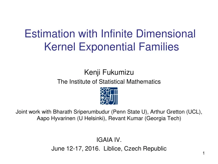
Estimation with Infinite Dimensional Kernel Exponential Families Kenji Fukumizu The Institute of Statistical Mathematics Joint work with Bharath Sriperumbudur (Penn State U), Arthur Gretton (UCL), Aapo Hyvarinen (U Helsinki), Revant Kumar (Georgia Tech) IGAIA IV. June 12-17, 2016. Liblice, Czech Republic 1

Introduction 2

Infinite dimensional exponential family  (Finite dim.) exponential family 𝑛 𝑞 𝜄 𝑦 = exp ෍ 𝜄 𝑘 𝑈 𝑘 𝑦 − 𝐵 𝜄 𝑟 0 (𝑦) 𝑘=1  Infinite dimensional extension? where 𝐵 𝑔 ≔ log ∫ 𝑓 𝑔(𝑦) 𝑟 0 𝑦 𝑒𝑦 𝑞 𝑔 𝑦 = exp 𝑔 𝑦 − 𝐵 𝑔 𝑟 0 (𝑦) 𝑔 is a natural parameter in an infinite dimensional function class. – Maximal exponential model (Pistone & Sempi AoS 1995) : • Orlicz space (Banach sp.) is used. • Estimation is not at all obvious. “Empirical” mean parameter cannot be defined.

 Kernel exponential manifold (Fukumizu 2009; Canu & Smola 2005) Reproducing kernel Hilbert space is used. • 𝑞 𝑔 𝑦 = exp 〈𝑔, 𝑙 ⋅, 𝑦 〉 − 𝐵 𝑔 𝑟 0 (𝑦) Infinite dimensional Parameter sufficient statistics • Empirical estimation is possible – Mean parameter: 𝑛 𝑔 = 𝐹 𝑞 𝑔 [𝑙 ⋅, 𝑌 ] 1 𝑜 – Maximum likelihood estimator: ෝ 𝑜 σ 𝑗=1 𝑛 𝑔 = 𝑙(⋅, 𝑌 𝑗 ) • Manifold structure can be defined (Fukumizu 2009) 4

Problems in estimation  Normalization constant / partition function – Even in finite dim. cases 𝑛 𝜄 𝑘 𝑈 𝑘 𝑦 𝑟 0 𝑦 𝑒𝑦 𝐵 𝜄 ≔ log ∫ 𝑓 σ 𝑘=1 is not easy to compute. – MLE: “Mean parameter  natural parameter” needs to solve 𝑜 𝜖𝐵 𝜄 = 1 𝑜 ෍ 𝑈 𝑌 𝑗 . 𝜖𝜄 𝑗=1 – Even more difficult for an infinite dimensional exponential family  This talk  score matching (Hyvarinen, JMLR 2005) – Estimation method without normalization constants. – Introducing a new method for (unnormalized) density estimation. 5

Score Matching 6

Score matching for exponential family (Hyvärinen, JMLR2005)  Fisher divergence 𝑒 𝑞, 𝑟 : two p.d.f.’s on Ω = ς 𝑏=1 𝑒 . (𝑡 𝑏 , 𝑢 𝑏 ) ⊂ 𝐒 ∪ ±∞ 𝑒 2 𝐾 𝑞||𝑟 ≔ 1 𝜖 log 𝑞 𝑦 − 𝜖 log 𝑟 𝑦 2 න ෍ 𝑞(𝑦)𝑒𝑦 𝜖𝑦 𝑏 𝜖𝑦 𝑏 𝑏=1 – 𝐾(𝑞| 𝑟 ≥ 0. Equality holds iff 𝑞 = 𝑟 (under mild conditions). – Derivative w.r.t. 𝑦 , not parameter. • For location parameter 𝑞(𝑦) = 𝑔 𝑦 − 𝜄 , 𝜖 log 𝑞 𝑦 = − 𝜖 log 𝑔 𝜄 𝑦 𝜖𝑦 𝑏 𝜖𝜄 𝑏 𝐾(𝑞||𝑟) = squared 𝑀 2 -distance of Fisher scores. 7

Set 𝑞 = 𝑞 0 (true), and 𝑟 = 𝑞 𝜄 to be estimated. 𝐾 𝜄 ≔ 𝐾 𝑞 0 ||𝑞 𝜄 2 𝜖 log 𝑞 𝜄 𝑦 − 𝜖 log 𝑞 0 𝑦 𝑒 1 2 ∫ σ 𝑏=1 = 𝑞 0 (𝑦)𝑒𝑦 𝜖𝑦 𝑏 𝜖𝑦 𝑏 ≡ ሚ 𝐾 𝜄 𝑒 𝜖 2 log 𝑞 𝜄 𝑦 𝑒 2 = 1 𝜖 log 𝑞 𝜄 𝑦 2 න ෍ 𝑞 0 (𝑦)𝑒𝑦 + න ෍ 𝑞 0 𝑦 𝑒𝑦 2 𝜖𝑦 𝑏 𝜖𝑦 𝑏 𝑏=1 𝑏=1 + const. 𝜖 log 𝑞 𝜄 𝑦 • 𝑦 𝑏 →𝑡 𝑏 or 𝑢 𝑏 𝑞 0 (𝑦) lim = 0 , and use partial integral Assume 𝜖𝑦 𝑏 𝑢 𝑏 𝜖 2 log 𝑞 𝜄 𝑦 𝜖 log 𝑞 𝜄 𝑦 𝜖 log 𝑞 0 𝑦 𝜖 log 𝑞 𝜄 𝑦 ∫ 𝑞 0 𝑦 𝑒𝑦 = 𝑞 0 𝑦 − ∫ 𝑞 0 (𝑦)𝑒𝑦 2 𝜖𝑦 𝑏 𝜖𝑦 𝑏 𝜖𝑦 𝑏 𝜖𝑦 𝑏 𝑡 𝑏 𝜖𝑞 0 𝑦 0 𝜖𝑦 𝑏 8

 Empirical estimation 𝑒 𝜖 2 log 𝑞 𝜄 𝑦 𝑒 2 𝐾 𝜄 = 1 𝜖 log 𝑞 𝜄 𝑦 ሚ 2 න ෍ 𝑞 0 (𝑦)𝑒𝑦 + න ෍ 𝑞 0 𝑦 𝑒𝑦 2 𝜖𝑦 𝑏 𝜖𝑦 𝑏 𝑏=1 𝑏=1 𝑌 1 , … , 𝑌 𝑜 : i.i.d. sample ~ 𝑞 0 . 𝑒 𝑜 2 + 𝜖 2 log 𝑞 𝜄 𝑌 𝑗 𝐾 𝑜 𝜄 = 1 1 𝜖 log 𝑞 𝜄 𝑌 𝑗 ሚ 𝑜 ෍ ෍ 2 2 𝜖𝑦 𝑏 𝜖𝑦 𝑏 𝑏=1 𝑗=1 መ 𝜄 = arg min ሚ 𝐾 𝑜 (𝜄) : Score matching estimator 9

Score matching for exponential family – For exponential family 𝑞 𝜄 𝑦 = exp σ 𝑘 𝜄 𝑘 𝑈 𝑘 𝑦 − 𝐵 𝜄 𝑟 0 𝑦 , ሚ 𝐾 𝑜 𝜄 2 𝑒 1 𝑜 𝑛 𝑛 + 𝜖 2 log 𝑟 0 𝑌 𝑗 𝜖 2 𝑈 𝜖𝑈 𝑘 𝑌 𝑗 + 𝜖 log 𝑟 0 𝑌 𝑗 𝑘 𝑌 𝑗 = ෍ ෍ ෍ 𝜄 + ෍ 𝜄 𝑘 𝑘 2 2 2 𝜖𝑦 𝑏 𝜖𝑦 𝑏 𝜖𝑦 𝑏 𝜖𝑦 𝑏 𝑗=1 𝑏=1 𝑘=1 𝑘=1 • No need of 𝐵 𝜄 ! (derivative w.r.t. 𝑦 ) • Quadratic form w.r.t. 𝜄  Solvable! • In the Gaussian case, ෠ 𝜄 is the same as MLE. 10

Kernel Exponential Family 11

Reproducing kernel Hilbert space – Def. Ω : set. 𝐼: Hilbert space consisting of functions on Ω . 𝐼 : reproducing kernel Hilbert space (RKHS), if for any 𝑦 ∈ Ω there is 𝑙 𝑦 ∈ 𝐼 s.t. 𝑔, 𝑙 𝑦 = 𝑔 𝑦 for ∀𝑔 ∈ 𝐼 [reproducing property] – 𝑙 𝑦, 𝑧 ≔ 𝑙 𝑦 (𝑧) . 𝑙 is a positive definite kernel, i.e., 𝑙 𝑦, 𝑧 = 𝑙(𝑧, 𝑦) and the Gram matrix 𝑙 𝑦 𝑗 , 𝑦 𝑘 𝑗𝑘 is positive semidefinite for any 𝑦 1 , … , 𝑦 𝑜 . – Moore-Aronszajn theorem: for any positive definite kernel on Ω , there uniquely exists an RKHS s.t. its reproducing kernel is 𝑙(⋅, 𝑦) . (One-to-one correspondence between p.d. kernel and RKHS) ‖𝑦−𝑧‖ 2 – Example of pos. def. kernel on 𝐒 𝑒 : 𝑙 𝑦, 𝑧 = exp − . 12 2𝜏 2

Kernel exponential family 𝑒 𝑒 . Def. 𝑙 : pos. def. kernel on Ω = ς 𝑏=1 (𝑡 𝑏 , 𝑢 𝑏 ) ⊂ 𝐒 ∪ ±∞ 𝐼 𝑙 : RKHS. 𝑟 0 : p.d.f. on Ω with supp 𝑟 0 = Ω . 𝐺 𝑙 ≔ {𝑔 ∈ 𝐼 𝑙 ∣ ∫ 𝑓 𝑔 𝑦 𝑟 0 𝑦 𝑒𝑦 < ∞} (functional) parameter space 𝑄 𝑙 ≔ {𝑞 𝑔 : Ω → 0, ∞ ∣ 𝑞 𝑔 𝑦 = 𝑓 𝑔 𝑦 −𝐵 𝑔 𝑟 0 𝑦 , 𝑔 ∈ 𝐺 𝑙 } where 𝐵 𝑔 ≔ ∫ 𝑓 𝑔(𝑦) 𝑟 0 𝑦 𝑒𝑦 𝑄 𝑙 : kernel exponential family (KEF) – With finite dimensional 𝐼 𝑙 , KEF is reduced to a finite dim. exponential family. e.g. 𝑙 𝑦, 𝑧 = 1 + 𝑦 𝑈 𝑧 2  Gaussian distributions. 13

Score matching for KEF Assume 𝑙 is of class 𝐷 2 ( 𝜖 𝑏+𝑐 𝑙(𝑦, 𝑧)/𝜖 𝑏 𝑦𝜖 𝑐 𝑧 exists and is continuous for 𝑏 + 𝑐 ≤ 2) and 𝜖 2 𝑙 𝑦,𝑧 lim ฬ 𝑞 0 𝑦 = 0 (for partial integral). 𝜖𝑦 𝑏 𝜖𝑧 𝑏 𝑧=𝑦 𝑦 𝑏 →𝑡 𝑏 or 𝑢 𝑏 – Score matching objective function 𝑒 1 𝑜 2 + 𝜖 2 log 𝑟 0 𝑌 𝑗 + 𝜖 2 𝑔 𝑌 𝑗 𝜖𝑔 𝑌 𝑗 + 𝜖 log 𝑟 0 𝑌 𝑗 ሚ 𝐾 𝑜 𝑔 ≔ ෍ ෍ 2 2 2 𝜖𝑦 𝑏 𝜖𝑦 𝑏 𝜖𝑦 𝑏 𝜖𝑦 𝑏 𝑗=1 𝑏=1 𝜖 2 𝑔 𝑌 𝑗 𝜖 2 𝑙 ⋅,𝑌 𝑗 𝜖𝑔 𝑌 𝑗 𝜖𝑙 ⋅,𝑌 𝑗 Note 𝑔 𝑌 𝑗 = 𝑔, 𝑙 ⋅, 𝑌 𝑗 , 𝜖𝑦 𝑏 = 𝑔, , = 𝑔, . 2 2 𝜖𝑦 𝑏 𝜖𝑦 𝑏 𝜖𝑦 𝑏 ሚ 𝐾 𝑜 𝑔 is a quadratic form w.r.t. 𝑔 ∈ 𝐼 . 14

– Estimation መ 𝐷 𝑜 𝑔 = 𝜊 𝑜 where 𝑒 𝜖𝑙 ⋅, 𝑌 𝑗 𝑜 𝐷 𝑜 ≔ 1 𝜖𝑙 ⋅, 𝑌 𝑗 መ 𝑜 ෍ ෍ ,∗ ∶ 𝐼 𝑙 → 𝐼 𝑙 𝜖𝑦 𝑏 𝜖𝑦 𝑏 𝑗=1 𝑏=1 𝑜 𝑒 + 𝜖 2 𝑙 ⋅, 𝑌 𝑗 𝜊 𝑜 ≔ 1 𝜖𝑙 ⋅, 𝑌 𝑗 𝜖 log 𝑟 0 𝑌 𝑗 መ 𝑜 ෍ ෍ ∈ 𝐼 𝑙 2 𝜖𝑦 𝑏 𝜖𝑦 𝑏 𝜖𝑦 𝑏 𝑗=1 𝑏=1 – Regularized estimator −1 መ ෡ መ 𝑔 𝑜 = 𝐷 𝑜 + 𝜇 𝑜 𝐽 𝜊 𝑜 i.e., ෡ 𝑜 = argmin 𝑔 ሚ 2 𝑔 𝐾 𝑜 𝑔 + 𝜇 𝑜 𝑔 𝐼 𝑙 15

Explicit Solution – Estimator: (from representer theorem) 𝑜 𝑒 𝜖𝑙 ⋅, 𝑌 𝑘 መ 𝑜 = 𝛽 መ 𝑔 𝜊 𝑜 + ෍ ෍ 𝛾 𝑘𝑐 𝜖𝑦 𝑐 𝑘=1 𝑐=1 where 2 1 1 𝑏 𝐻 𝑗𝑘 𝑏𝑐 + 𝜇 ℎ 𝑘 𝑏 2 + 𝜇 መ 𝑐 2 𝑜 σ 𝑏,𝑗 ℎ 𝑗 𝑜 σ 𝑏,𝑗 ℎ 𝑗 𝜊 𝑜 መ 𝛽 𝜊 𝑜 𝛾 𝑗𝑏 = − 𝑏 𝐻 𝑗𝑘 𝑏𝑐 + 𝜇 ℎ 𝑘 𝑐𝑑 + 𝜇 𝐻 𝑗𝑘 1 1 𝑐 𝑐 𝑏𝑑 𝐻 𝑛𝑘 𝑏𝑐 ℎ 𝑘 𝑜 σ 𝑏,𝑗 ℎ 𝑗 𝑜 σ 𝑑,𝑛 𝐻 𝑗𝑛 𝜖 3 𝑙 𝑌 𝑗 ,𝑌 𝑘 𝜖 2 𝑙 𝑌 𝑗 ,𝑌 𝑘 𝑐 = 1 𝜖ℓ 𝑌 𝑗 𝜖ℓ 𝑌 𝑗 𝜖 log 𝑟 0 𝑌 𝑗 𝑜 σ 𝑗,𝑏 ℎ 𝑘 2 𝜖𝑧 𝑐 + 𝜖𝑦 𝑏 , 𝜖𝑦 𝑏 = 𝜖𝑦 𝑏 𝜖𝑦 𝑏 𝜖𝑧 𝑐 𝜖𝑦 𝑏 𝜖 2 𝑙 𝑌 𝑗 ,𝑌 𝑘 2 = 𝜖 4 𝑙 𝑌 𝑗 ,𝑌 𝑘 𝜖 3 𝑙 𝑌 𝑗 ,𝑌 𝑘 𝜖 2 𝑙 𝑌 𝑗 ,𝑌 𝑘 𝜖ℓ(𝑌 𝑘 ) 𝜖ℓ(𝑌 𝑘 ) 𝑏𝑐 = 1 𝜖ℓ 𝑌 𝑗 𝜖𝑦 𝑏 𝜖𝑧 𝑐 , መ 𝐻 𝑗𝑘 𝜊 𝑜 𝑜 2 σ 𝑗𝑘,𝑏𝑐 2 + 2 𝜖𝑦 𝑐 + 2 𝜖𝑧 𝑐 2 𝜖𝑧 𝑐 𝜖𝑦 𝑏 𝜖𝑦 𝑏 𝜖𝑦 𝑏 𝜖𝑧 𝑐 𝜖𝑦 𝑏 𝜖𝑦 𝑐 𝜖𝑙 ⋅,𝑌 𝑘 መ , መ • 𝑔 𝜊 𝑜 . 𝑜 can be taken in Span 𝜖𝑦 𝑐 • Estimator is simply given by solving 1 + 𝑜𝑒 -dimensional linear 16 equation.

Unnormalized p.d.f. – Score matching for KEF gives only 𝑔(𝑦) or 𝑓 𝑔 𝑦 , unnormalized p.d.f. • Estimation of 𝐵 𝑔 ≔ ∫ 𝑓 𝑔(𝑦) 𝑟 0 𝑦 𝑒𝑦 is yet nontrivial. – There are interesting applications. 1) Nonparametric structure learning for graphical model given data (Sun, Kolar, Xu NIPS2015) 𝑞 𝑌 ∝ ෑ 𝑞 𝑗𝑘 𝑌 𝑗 , 𝑌 𝑘 , 𝐻 = (𝑊, 𝐹) 𝑗𝑘∈𝐹 𝑞 𝑗𝑘 is estimated nonparametrically with KEF (with sparse edges). a b c d 17 e