Estimation of the survival function Rasmus Waagepetersen Department - PowerPoint PPT Presentation
Estimation of the survival function Rasmus Waagepetersen Department of Mathematics Aalborg University Denmark October 29, 2020 1 / 23 Estimation of the survival function - actuarial estimate Suppose we are given data in terms of a lifetable
Estimation of the survival function Rasmus Waagepetersen Department of Mathematics Aalborg University Denmark October 29, 2020 1 / 23
Estimation of the survival function - actuarial estimate Suppose we are given data in terms of a lifetable for a population. That is, for fixed times 0 = u 0 < u 1 < u 2 < · · · we know for each u i ◮ the number r ( u i ) of individuals at risk (not dead or censored) at time u i (i.e. both survival time and censoring time ≥ u i ) ◮ the number of deaths d i in the interval [ u i − 1 ; u i [ and ◮ the number c i of censorings in [ u i − 1 ; u i [. Note: r ( u i ) = r ( u i − 1 ) − d i − c i and initial population size n = r ( u 0 ) 2 / 23
We want to estimate P ( X ≥ u i ) Usual estimate: P ( X ≥ u i ) = #alive up to time u i ˆ n If no censoring: P ( X ≥ u i ) = r ( u i ) ˆ n Problem: due to censoring we often do not know numerator - typically larger than r ( u i ) ! (individuals censored prior to u i may well be alive) 3 / 23
Factorization l � P ( X ≥ u l ) = P ( X ≥ u k | X ≥ u k − 1 ) = k =1 l l � � (1 − P ( X < u k | X ≥ u k − 1 )) = (1 − p k ) k =1 k =1 Here p k is the probability of dying in the k th interval given alive at start of interval. If no censoring then d k p k = ˆ r ( u k − 1 ) If censoring takes place in the k th interval then numerator too small - or denominator too large. Idea: we modify denominator. 4 / 23
Suppose all censoring takes place in the very beginning of the k th interval at time u k − 1 . Then the effective number at risk in the k th interval is r ( u k − 1 ) − c k and we let d k p k = ˆ r ( u k − 1 ) − c k If all censoring takes place at the very end of the interval then d k p k = ˆ r ( u k − 1 ) If the censoring times are uniformly dispersed on the interval then a censored individual is at risk on average half of the interval and we use d k p k = ˆ r ( u k − 1 ) − c k / 2 I.e. the so-called actuarial estimate - uses denominator given by average of previous denominators. 5 / 23
Resulting estimate: l � P ( X ≥ u l ) = (1 − ˆ p k ) k =1 Note: ˆ p k = 0 if no deaths in the k th interval ! 6 / 23
Censoring assumptions Requirement: individuals contributing to the denominator must be representative of those alive at time u k − 1 . Thus the probability that a person dies in [ u k − 1 ; u k [ given that the person is at risk (not dead or censored) at time u k − 1 must coincide with p k . In other words, c k should represent a random sample of the r ( u k − 1 ) persons at risk. E.g. problematic if persons are censored because they appear very weak at time u k − 1 . (This is related to what we called independent censoring (or non-informative censoring in KM, unfortunately terminology is not consistent over text books) Then the persons at risk at time u k − 1 are also representative of those who are alive at time u k − 1 . 7 / 23
Estimation using exact death times - reduced sample estimator Suppose now we have observed the exact death or censoring times ( t i , δ i ) and we want to estimate P ( X > t ) for an arbitrary t . Suppose the censoring times C i are all observed and independent of the death times X i (e.g. type 1 censoring). Unbiased reduced sample estimator: � n i =1 1[ x i > t , c i > t ] ˆ S red ( t ) = � n i =1 1[ c i > t ] Problem: inefficient use of observations. An observation censored at time u does not contribute to ˆ S red ( t ) for t ≥ u . Not applicable in case of competing risks when C i > t not observed if death happens prior to t . 8 / 23
Alternative idea: introduce discretization 0 = u 1 < u 2 < · · · < u L = t and apply actuarial estimate. Next consider limit L → ∞ and u k − u k − 1 → 0 (finer and finer discretization). Assume also that no censoring time coincides with a death time. Let D denote the set of distinct death times and let d ( t ∗ ) denote the number of deaths at time t ∗ for t ∗ ∈ D . Then, for L sufficiently large, there is a most one distinct death time in each interval and if there is a death time then there is no censoring. 9 / 23
Thus we have two possibilities ˆ p k = 0 (no death) or p k = d ( t ∗ ) ˆ r ( t ∗ ) if t ∗ is the unique death time falling in [ u k − 1 ; u k [. Thus our estimate becomes (1 − d ( t ∗ ) ˆ � P ( X ≥ t ) = r ( t ∗ ) ) t ∗ ∈ D : t ∗ < t and (1 − d ( t ∗ ) S ( t ) = ˆ ˆ � P ( X > t ) = r ( t ∗ ) ) t ∗ ∈ D : t ∗ ≤ t This is the Kaplan-Meier (product limit) estimate. Estimate is right-continuous. If last event, say t n , is a death then ˆ S ( t ) = 0 for t ≥ t n . If last event is a censoring then ˆ S ( t ) = ˆ S ( t n ) > 0 for t ≥ t n . 10 / 23
Nelson-Aalen estimator of cumulative hazard � t L L � � H ( t ) = h ( u ) d u ≈ h ( u k − 1 )[ u k − u k − 1 ] ≈ p k 0 k =1 k =1 Thus L ˆ � H ( t ) = ˆ p k k =1 In the limit (Nelson-Aalen estimator) d ( t ∗ ) ˆ � H ( t ) = r ( t ∗ ) t ∗ ∈ D : t ∗ ≤ t Recall S ( t ) = exp( − H ( t )). Estimates ˆ H ( t ) and ˆ S ( t ) related by log(1 − x ) ≈ − x or exp( − x ) ≈ 1 − x for x close to 0. 11 / 23
Asymptotic results Consider the random censoring case where the n survival and censoring times X i and C i , i = 1 , . . . , n have survival functions S and G . Consider any 0 < v < ∞ with S ( v ) > 0, assume that 1 − S is absolute continous with density f and that G is continuous. Then the random function √ n ( ˆ S ( t ) − S ( t )) , 0 < t < v converges in distribution to a zero mean Gaussian process { R ( u ) } 0 < u < v with covariance function � min( t 1 , t 2 ) h ( u ) C ov ( R ( t 1 ) , R ( t 2 )) = S ( t 1 ) S ( t 2 ) S ( u ) G ( u ) d u 0 (see e.g. Lawless, 1982). 12 / 23
Implications of asymptotic result For any 0 < t < v : � t S ( t ) ≈ N ( S ( t ) , σ 2 h ( u ) ˆ n ) with σ 2 t t = S ( t ) 2 S ( u ) G ( u ) d u 0 √ n -consistency: for any fixed c , P ( √ n | ˆ S ( t ) − S ( t ) | /σ t < c ) converges to 1 − 2Φ( − c ). Loosely speaking, √ n ( ˆ S ( t ) − S ( t )) is bounded with probability 1, S ( t ) − S ( t ) converges to zero as 1 / √ n . thus ˆ 95% Confidence interval (pointwise !): S ( t ) ± 1 . 96 σ t / √ n ˆ 13 / 23
Estimation of asymptotic variance In practice we need to estimate asymptotic variance σ 2 t : L L h ( u k − 1 ) n σ 2 t ≈ S ( t ) 2 � S ( u k − 1 ) G ( u k − 1 )( u k − u k − 1 ) ≈ S ( t ) 2 � ˆ p k r ( u k − 1 ) k =1 k =1 Taking the limit L → ∞ as before we obtain σ 2 d ( t ∗ ) ˆ 1 n = ˆ S ( t ) 2 � t r ( t ∗ ) r ( t ∗ ) t ∗ ∈ D : t ∗ ≤ t Typically, the closely related Greenwoods formula is used: σ 2 d ( t ∗ ) ˆ 1 n = ˆ t S ( t ) 2 � r ( t ∗ ) r ( t ∗ ) − d ( t ∗ ) t ∗ ∈ D : t ∗ ≤ t p k is either 0 or d ( t ∗ ) / r ( t ∗ ) and in (recall: for L sufficiently large ˆ the latter case, r ( u k ) = r ( t ∗ ) − d ( t ∗ )) 14 / 23
Note: Greenwood’s formula can be derived by heuristic arguments using L ˆ � S ( t ) = (1 − ˆ p k ) = g (ˆ p 1 , . . . , ˆ p L ) k =1 where g ( x 1 , . . . , x L ) = � L i =1 (1 − x i ) and the δ -method. We also assume ˆ p k uncorrelated and estimate V ar ˆ p k by p k (1 − ˆ ˆ p k ) / r ( u k − 1 ) - see next slide. 15 / 23
Some remarks on the ˆ p k Consider for simplicity the case with no censoring. Let k � N k = d k l =1 be counting process of deaths. d k = N k − N k − 1 , r ( u k ) = n − N k . Assume d k | N 1 , . . . , N k − 1 ∼ bin( r ( u k − 1 ) , p k ). Then E [ˆ p k − p k | N 1 , . . . , N k − 1 ] = 0 . p k | N 1 , . . . , N k − 1 ]] = p k and for k ′ > k , This implies E [ˆ p k ] = E [ E [ˆ C ov [ˆ p k , ˆ p k ′ ] = E [(ˆ p k − p k ) E [ˆ p k ′ − p k ′ | N 1 , . . . , N k ′ − 1 ]] = 0 Thus ˆ p k ’s uncorrelated. 16 / 23
Moreover, V ar ˆ p k = V ar [ E [ˆ p k | N 1 , . . . , N k − 1 ] + EV ar [ˆ p k | N 1 , . . . , N k − 1 ]] = 0 + E [ p k (1 − p k ) / r ( u k − 1 )] So we may estimate V ar ˆ p k by p k (1 − ˆ ˆ p k ) / r ( u k − 1 ) Note M k = N k − � k l =1 p l r ( u l − 1 ) is a martingale with respect to ‘history’ N 1 , . . . , N k − 1 : E [ M k | N 1 , . . . , N k − 1 ] = M k − 1 + E [ d k − r ( u k − 1 ) p k | r ( u k − 1 )] = M k − 1 This implies uncorrelated increments M k − M k − 1 . M k is centered/compensated version of N k : E [ M k ] = E [ M k − 1 ] = . . . = E [ M 1 ] = 0 17 / 23
Confidence intervals Issues: 0 ≤ S ( t ) ≤ 1. This is not respected by previously mentioned confidence intervals. KM discusses various solutions including deriving confidence interval based on transformed S ( t ) and transforming back. KM section 4.4 also discusses simultaneous confidence bands. 18 / 23
log( − log( · ))-transformation L ( t ) = log( H ( t )) = log( − log( S ( t )) is a function on R (unrestricted). Let ˆ L ( t ) = log( − log( ˆ S ( t )) with standard error σ L . Then approximate 95% confidence interval for L ( t ) is [ˆ L ( t ) − 2 σ L ; ˆ L ( t ) + 2 σ L ] . Transforming back we obtain approximate 95% interval for S ( t ): [( ˆ S ( t )) exp( − 2 σ L ) ; ( ˆ S ( t )) exp(+2 σ L ) ] . Finally, by δ -method, σ L ≈ std.err( ˆ S ( t )) / (log( ˆ S ( t )) ˆ S ( t )) See KM (4.3.2). 19 / 23
Recommend
More recommend
Explore More Topics
Stay informed with curated content and fresh updates.
