Estimating Risk under Estimating statistics . . . Linearized - PowerPoint PPT Presentation
Computing statistics is . . . Additional problem: . . . Traditional approach . . . Estimating Risk under Estimating statistics . . . Linearized techniques Interval Uncertainty: The exact estimation . . . Need for parallelization Sequential
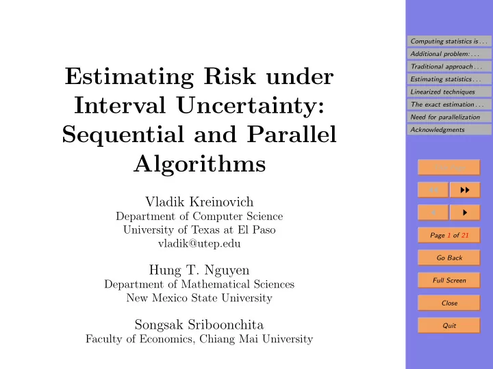
Computing statistics is . . . Additional problem: . . . Traditional approach . . . Estimating Risk under Estimating statistics . . . Linearized techniques Interval Uncertainty: The exact estimation . . . Need for parallelization Sequential and Parallel Acknowledgments Algorithms Title Page ◭◭ ◮◮ Vladik Kreinovich ◭ ◮ Department of Computer Science University of Texas at El Paso Page 1 of 21 vladik@utep.edu Go Back Hung T. Nguyen Full Screen Department of Mathematical Sciences New Mexico State University Close Songsak Sriboonchita Quit Faculty of Economics, Chiang Mai University
Computing statistics is . . . 1. Computing statistics is important Additional problem: . . . • Problem: estimating the quality of of an individual in- Traditional approach . . . vestment – and of the investment portfolio. Estimating statistics . . . Linearized techniques • Traditional econometrics approach: use expected re- The exact estimation . . . turn and its risk (variance). Need for parallelization • How to estimate these characteristics: Acknowledgments – trace the past returns x 1 , . . . , x n of a given (and/or Title Page similar) investment; ◭◭ ◮◮ – compute the statistical characteristics based on these ◭ ◮ returns. n Page 2 of 21 � • The expected return: E = 1 n · x i . Go Back i =1 Full Screen n � • The risk: V = 1 ( x i − E ) 2 . n · Close i =1 Quit
Computing statistics is . . . 2. Additional problem: interval uncertainty Additional problem: . . . • The return (per unit investment) is defined as Traditional approach . . . Estimating statistics . . . – the selling price of the corresponding financial in- Linearized techniques strument at the end of, e.g., a one-year period, The exact estimation . . . – divided by the buying price of this instrument at Need for parallelization the beginning of this period. Acknowledgments • It is usually assumed that we know the exact values Title Page x 1 , . . . , x n of the returns. ◭◭ ◮◮ • In practice, however, both the selling and the buying ◭ ◮ prices unpredictably fluctuate within a single day. Page 3 of 21 • These minute-by-minute fluctuations are not always Go Back recorded. Full Screen • What we usually have recorded is the daily range of prices [ x i , x i ]. Close Quit
Computing statistics is . . . 3. Traditional approach to solving the problem of in- Additional problem: . . . terval uncertainty Traditional approach . . . • Traditional approach: Estimating statistics . . . x i = x i + x i Linearized techniques – take the average � and 2 The exact estimation . . . – compute the characteristics based on these aver- Need for parallelization ages. Acknowledgments • Resulting estimate for the expected return: Title Page n � ◭◭ ◮◮ E = 1 � n · � x i , ◭ ◮ i =1 Page 4 of 21 • Resulting estimate for the risk: Go Back � � 2 n n n � � � V = 1 E ) 2 = 1 1 x i ) 2 − � x i − � Full Screen n · ( � n · ( � n · x i � . i =1 i =1 i =1 Close Quit
Computing statistics is . . . 4. Traditional approach: limitations Additional problem: . . . • In the bull market: Traditional approach . . . Estimating statistics . . . – there may be dips leading to a small value of x i , Linearized techniques – but overall, the values are increasing and The exact estimation . . . – therefore, x i is a reasonable estimate for x i , and � x i Need for parallelization underestimates the high price x i . Acknowledgments • In the bear market: Title Page – spikes are accidental but lower values are typical, ◭◭ ◮◮ – therefore, x i is a reasonable estimate for x i , and � x i ◭ ◮ overestimates the low price x i . Page 5 of 21 • So, we underestimate the low prices and underestimate Go Back the high prices. Full Screen • Thus we underestimate the variance (the measure of Close price variation). Quit
Computing statistics is . . . 5. Estimating statistics under interval uncertainty: a Additional problem: . . . computational problem Traditional approach . . . • Traditional assumption: we know the true values x 1 , . . . , x n . Estimating statistics . . . Linearized techniques • Traditional computations: estimate the value of a sta- The exact estimation . . . tistical characteristic C ( x 1 , . . . , x n ). Need for parallelization • Interval uncertainty: we only know the intervals x 1 = Acknowledgments [ x 1 , x 1 ] , . . . , x n = [ x n , x n ] that contain x i . Title Page • Fact: different values x i ∈ x i lead, in general, to dif- ◭◭ ◮◮ ferent values of C ( x 1 , . . . , x n ). ◭ ◮ • Conclusion: we need to estimate the range Page 6 of 21 def C ( x 1 , . . . , x n ) = { C ( x 1 , . . . , x n ) | x 1 ∈ x 1 , . . . , x n ∈ x n } . Go Back • Computational challenge: modify the existing statisti- Full Screen cal algorithms so that they compute these ranges. Close Quit
Computing statistics is . . . 6. Estimating expected return under interval uncer- Additional problem: . . . tainty Traditional approach . . . • Fact: the expected return (arithmetic average) E is a Estimating statistics . . . monotonically increasing function of x 1 , . . . , x n . Linearized techniques The exact estimation . . . • Conclusions: Need for parallelization – the smallest possible value E is attained when each Acknowledgments value x i is the smallest possible ( x i = x i ); Title Page – the largest possible value is attained when x i = x i ◭◭ ◮◮ for all i . ◭ ◮ • In other words, the range E of E is equal to Page 7 of 21 [ E ( x 1 , . . . , x n ) , E ( x 1 , . . . , x n )] . Go Back • In other words, E = 1 n · ( x 1 + . . . + x n ) and Full Screen E = 1 Close n · ( x 1 + . . . + x n ). Quit
Computing statistics is . . . 7. Linearized techniques Additional problem: . . . • Idea: when the daily fluctuations are small, we can use Traditional approach . . . the linearization techniques: Estimating statistics . . . Linearized techniques – we represent the values x i as x i = � x i + ∆ x i , where def The exact estimation . . . the differences ∆ x i = x i − � x i are small, and Need for parallelization – we ignore quadratic terms in the formula for the Acknowledgments variance. Title Page • Details: the condition that x i ∈ [ x i , x i ] means that = x i − x i ◭◭ ◮◮ def ∆ x i ∈ [ − ∆ i , ∆ i ], where ∆ i . 2 ◭ ◮ • General case: Page 8 of 21 � n ∂C C ( x 1 , . . . , x n ) ≈ C ( � x 1 , . . . , � x n )+ ( � x 1 , . . . , � x n ) · ∆ x i . Go Back ∂x i i =1 � � 2 Full Screen n n � � • Case study: the variance V = 1 1 x 2 n · i − n · Close x i . i =1 i =1 Quit
Computing statistics is . . . 8. Linearization (cont-d) Additional problem: . . . � n Traditional approach . . . • Formula: V = � x i − � V + 2 ( � E ) · ∆ x i . Estimating statistics . . . i =1 • The expression for V is monotonic in each ∆ x i ∈ [ − ∆ i , ∆ i ]: Linearized techniques The exact estimation . . . x i ≥ � – it is increasing when � E and Need for parallelization x i ≤ � – it is decreasing when � E . Acknowledgments x i ≥ � • When � E : maximum is attained when ∆ x i = ∆ i ; Title Page x i − � the corresponding term in V is ( � E ) · ∆ i . ◭◭ ◮◮ x i ≤ � • When � E : maximum is attained when ∆ x i = − ∆ i ; ◭ ◮ x i − � the corresponding term in V is − ( � E ) · ∆ i . Page 9 of 21 x i − � • General expression: | � E | · ∆ i . Go Back • Conclusion: the range of V is [ � V − 2∆ , � V +2∆], where Full Screen n � def x i − � ∆ = | � E | · ∆ i . Close i =1 Quit
Computing statistics is . . . 9. Linearization approximation is not always adequate Additional problem: . . . • In finance, the gain is often obtained by a small (often Traditional approach . . . < 1%) advantage. Estimating statistics . . . Linearized techniques • From this viewpoint, it is desirable to have estimates The exact estimation . . . which are as accurate as possible. Need for parallelization • When the situation is stable, the daily fluctuations are Acknowledgments low, and quadratic terms can be reasonable ignored. Title Page • However, the whole purpose of estimating risk is to ◭◭ ◮◮ cover situations with high volatility. ◭ ◮ • In such situations, the daily fluctuations x i − x i = 2∆ i can also be sizeable. Page 10 of 21 • Thus, terms quadratic in ∆ i cannot be ignored if we Go Back want accurate estimates. Full Screen • In such situations, we need the exact range of the vari- Close ance (risk) V . Quit
Computing statistics is . . . 10. The exact estimation of risk under interval uncer- Additional problem: . . . tainty is, in general, an NP-hard problem Traditional approach . . . • Computational problem (reminder): Estimating statistics . . . Linearized techniques – given: interval data x i ∈ [ x i , x i ]; The exact estimation . . . – compute: the exact range V = [ V , V ] for the risk Need for parallelization (variance) V . Acknowledgments • Fact: this problem is, in general, computationally dif- Title Page ficult (NP-hard). ◭◭ ◮◮ • Specifically: ◭ ◮ – there is a O ( n · log( n )) time algorithm for computing Page 11 of 21 V , but Go Back – computing V is, in general, NP-hard. Full Screen Close Quit
Recommend
More recommend
Explore More Topics
Stay informed with curated content and fresh updates.
