Enhancing Voxel Carving by Capture Volume Calculations - PowerPoint PPT Presentation
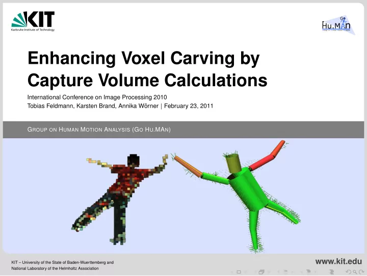
Group on Human Motion Analysis Enhancing Voxel Carving by Capture Volume Calculations International Conference on Image Processing 2010 Tobias Feldmann, Karsten Brand, Annika W orner | February 23, 2011 G ROUP ON H UMAN M OTION A NALYSIS (G O
Group on Human Motion Analysis Enhancing Voxel Carving by Capture Volume Calculations International Conference on Image Processing 2010 Tobias Feldmann, Karsten Brand, Annika W¨ orner | February 23, 2011 G ROUP ON H UMAN M OTION A NALYSIS (G O H U .MA N ) www.kit.edu KIT – University of the State of Baden-Wuerttemberg and National Laboratory of the Helmholtz Association
Outline Introduction 1 Basics 2 Clipping Polygons With Half Spaces Contribution 3 Polyhedron, View Frustum and Adjacency Matrix Polyhedron clipping Problems in the real world Volume calculations Evaluation 4 Conclusion 5 Introduction Basics Contribution Evaluation Conclusion February 23, 2011 2/27 Tobias Feldmann, Karsten Brand, Annika W¨ orner – Capture Volume Calculations
Introduction Dense volumetric reconstruction of gymnasts in sports. Multi camera based voxel carving approach. Introduction Basics Contribution Evaluation Conclusion February 23, 2011 3/27 Tobias Feldmann, Karsten Brand, Annika W¨ orner – Capture Volume Calculations
Problem Statement During voxel based 3d reconstruction one question directly arises: Question: Which size for the reconstruction area? Introduction Basics Contribution Evaluation Conclusion February 23, 2011 4/27 Tobias Feldmann, Karsten Brand, Annika W¨ orner – Capture Volume Calculations
Problem Statement During voxel based 3d reconstruction one question directly arises: Question: Which size for the reconstruction area? Answer: Bounding box of clipping polyhedron of all camera frusta. Introduction Basics Contribution Evaluation Conclusion February 23, 2011 4/27 Tobias Feldmann, Karsten Brand, Annika W¨ orner – Capture Volume Calculations
Quick review of half spaces Hyper plane E defined by three points a ,� c ∈ R 3 . � b ,� Normal � n and distance to origin d E : n = ( � � b − � a ) × ( � c − � d E = � � n ,� a ) , a � Plane E : x ∈ R 3 E : � � n ,� � x � = d with Hesse normal form: � n d � n 0 = � d � , d 0 = � d � Distance of a point � p ∈ R 3 : p = � � n 0 ,� d E ,� p � − d 0 Half space H 1 defined by hyperplane E with normal � n . Each point � p with positive or zero distance to E is ∈ H 1 . Introduction Basics Contribution Evaluation Conclusion February 23, 2011 5/27 Tobias Feldmann, Karsten Brand, Annika W¨ orner – Capture Volume Calculations
Clipping polygons with planes Goal : Clipping camera view polygons with each other. Approach: Sutherland & Hodgman [1]. Introduction Basics Contribution Evaluation Conclusion February 23, 2011 6/27 Tobias Feldmann, Karsten Brand, Annika W¨ orner – Capture Volume Calculations
Clipping polygons with planes Goal : Clipping camera view polygons with each other. Approach: Sutherland & Hodgman [1]. Introduction Basics Contribution Evaluation Conclusion February 23, 2011 6/27 Tobias Feldmann, Karsten Brand, Annika W¨ orner – Capture Volume Calculations
Sutherland & Hodgman Algorithm Published 1974 by Ivan E. Sutherland and Gary W. Hodgman in [1]. Algorithm is able to clip an arbitrary start polygon with an convex clip polygon : Treat start polygon as sorted set of points. 1 Split clip polygon into edges. 2 Check distance of all points to each clipping edge. 3 Create target polygon from points with positive distance 4 and points of intersection with clipping edges. Edge definition implicitly by order of positive and intersection points. Introduction Basics Contribution Evaluation Conclusion February 23, 2011 7/27 Tobias Feldmann, Karsten Brand, Annika W¨ orner – Capture Volume Calculations
Clipping Example - Step I A and B both have a positive distance to E . ⇒ B added to new polygon (green dot). Introduction Basics Contribution Evaluation Conclusion February 23, 2011 8/27 Tobias Feldmann, Karsten Brand, Annika W¨ orner – Capture Volume Calculations
Clipping Example - Step II B has positive distance, C has negative distance to E . ⇒ Intersection point BC added to new polygon (green dot). Introduction Basics Contribution Evaluation Conclusion February 23, 2011 8/27 Tobias Feldmann, Karsten Brand, Annika W¨ orner – Capture Volume Calculations
Clipping Example - Step III C and D both have a negative distance. ⇒ No point added to new polygon. Introduction Basics Contribution Evaluation Conclusion February 23, 2011 8/27 Tobias Feldmann, Karsten Brand, Annika W¨ orner – Capture Volume Calculations
Clipping Example - Step IV D has negative distance, A has positive distance to E . ⇒ Intersection point DA and A added to polygon. Introduction Basics Contribution Evaluation Conclusion February 23, 2011 8/27 Tobias Feldmann, Karsten Brand, Annika W¨ orner – Capture Volume Calculations
Contribution Let’s go into 3d now! Introduction Basics Contribution Evaluation Conclusion February 23, 2011 9/27 Tobias Feldmann, Karsten Brand, Annika W¨ orner – Capture Volume Calculations
Polyhedron and View Frustum Polyhedron: A geometric solid in 3d with flat faces defined by points or straight edges. Frustum: Subtype of polyhedron. Apex A defines camera center, ground BCDE defines far plane. List representation of the faces: A B C A D C A E D A B E B C D E Introduction Basics Contribution Evaluation Conclusion February 23, 2011 10/27 Tobias Feldmann, Karsten Brand, Annika W¨ orner – Capture Volume Calculations
Problem definition What do we want to do next? Sutherland & Hodgman Algorithm has to be extended to 3d polyhedrons: Clipping of a view frustum ABCDE with a plane H in 3d. Introduction Basics Contribution Evaluation Conclusion February 23, 2011 11/27 Tobias Feldmann, Karsten Brand, Annika W¨ orner – Capture Volume Calculations
Sutherland & Hodgman in 3d Problem: In 3d no unique direction along the edges to traverse the start polyhedron. Two possible solutions: Treat faces as polygons. 1 Drawback: Similar intersection points might occur due to numerical precision multiple times and merging is error prone. Run along the points instead of the faces. 2 Drawback: Edges will get lost. Edges can be reconstructed easily with the Quickhull algorithm [2]. ⇒ Polyhedron is traversed along the points. Introduction Basics Contribution Evaluation Conclusion February 23, 2011 12/27 Tobias Feldmann, Karsten Brand, Annika W¨ orner – Capture Volume Calculations
Sutherland & Hodgman in 3d Problem: In 3d no unique direction along the edges to traverse the start polyhedron. Two possible solutions: Treat faces as polygons. 1 Drawback: Similar intersection points might occur due to numerical precision multiple times and merging is error prone. Run along the points instead of the faces. 2 Drawback: Edges will get lost. Edges can be reconstructed easily with the Quickhull algorithm [2]. ⇒ Polyhedron is traversed along the points. Introduction Basics Contribution Evaluation Conclusion February 23, 2011 12/27 Tobias Feldmann, Karsten Brand, Annika W¨ orner – Capture Volume Calculations
Sutherland & Hodgman in 3d Problem: In 3d no unique direction along the edges to traverse the start polyhedron. Two possible solutions: Treat faces as polygons. 1 Drawback: Similar intersection points might occur due to numerical precision multiple times and merging is error prone. Run along the points instead of the faces. 2 Drawback: Edges will get lost. Edges can be reconstructed easily with the Quickhull algorithm [2]. ⇒ Polyhedron is traversed along the points. Introduction Basics Contribution Evaluation Conclusion February 23, 2011 12/27 Tobias Feldmann, Karsten Brand, Annika W¨ orner – Capture Volume Calculations
Point Traversal via Adjacency Matrix A B C A D C A E D A B E B C D E List of faces. Introduction Basics Contribution Evaluation Conclusion February 23, 2011 13/27 Tobias Feldmann, Karsten Brand, Annika W¨ orner – Capture Volume Calculations
Point Traversal via Adjacency Matrix A B C 0 1 1 1 1 A D C 1 0 1 0 1 A E D 1 1 0 1 0 A B E 1 0 1 0 1 B C D E 1 1 0 1 0 List of faces. Full adjacency matrix (undirected graph). If edge between points i , j , then 1, else 0 into adjacency matrix. Introduction Basics Contribution Evaluation Conclusion February 23, 2011 13/27 Tobias Feldmann, Karsten Brand, Annika W¨ orner – Capture Volume Calculations
Point Traversal via Adjacency Matrix A B C 0 1 1 1 1 A D C 1 0 1 0 1 A E D 1 1 0 1 0 A B E 1 0 1 0 1 B C D E 1 1 0 1 0 List of faces. Full adjacency matrix (undirected graph). If edge between points i , j , then 1, else 0 into adjacency matrix. Upper triangle contains directed graph for edge traversal. Introduction Basics Contribution Evaluation Conclusion February 23, 2011 13/27 Tobias Feldmann, Karsten Brand, Annika W¨ orner – Capture Volume Calculations
Recommend


More recommend
Explore More Topics
Stay informed with curated content and fresh updates.