Enhancing constraints on modified gravity and inflation with - PowerPoint PPT Presentation

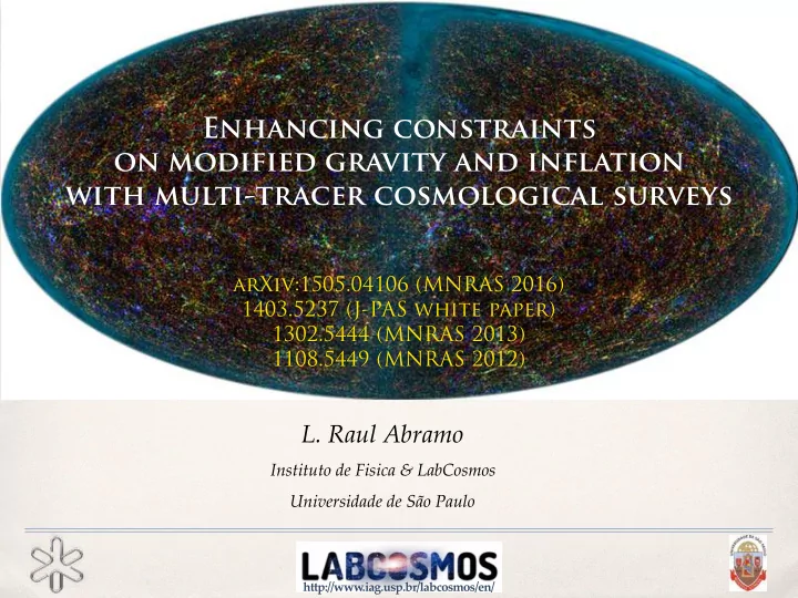
Enhancing constraints on modified gravity and inflation with multi-tracer cosmological surveys arXiv:1505.04106 (MNRAS 2016) 1403.5237 (J-PAS white paper) 1302.5444 (MNRAS 2013) 1108.5449 (MNRAS 2012) L. Raul Abramo Instituto de Fisica & LabCosmos Universidade de São Paulo http://www.iag.usp.br/labcosmos/en/

Galaxy surveys are evolving We used to live in an We are now in the age of era of shot (“counts”) noise cosmic variance and systematics SDSS [ Finding galaxies was the limiting factor] [ Volume and control are the limiting factors]

Surveys of large-scale structure are now limited by cosmic variance and systematics Anderson et al. [BOSS] 1312.4877 P ( k ) /P dewig ( k ) However, up to any given redshift there is only a finite volume. Moreover, we are reaching closer to the limits of the observable Universe!

Shot noise: finite number of counts of the tracers of the underlying density field (Poisson statistics) Cosmic variance: finite volume inside which we can estimate the amplitudes and phases of the (Gaussian) random modes of the density field k ) + 1 P g ( ~ g P m ( ~ k ) ' b 2 ¯ n g n g P g ( ~ g P m ( ~ n g b 2 Clustering in units of shot noise ¯ k ) ' ¯ k ) + 1 SNR noise

Feldman, Kaiser & Peacock 1994 ( FKP ) Tegmark et al. 1997, 1998 Fisher information of galaxy surveys $$$ ◆ 2 1 + P g 1.00 P g Cosmic Variance 0.50 shot noise happiness ✓ 0.20 Information ∼ L 0.10 0.05 0.02 0.01 0.1 0.5 1.0 5.0 10.0 50.0 P g more galaxies Signal/Noise: ⇤ 2 G 2 ( z ) P m ( k ) Clustering strength x, ~ b g ( z, k ) + f ( z ) µ 2 ⇥ P g ( ~ k ) ≡ ¯ n g ( ~ x ) of galaxy type “ g” in k redshift space

FKP 1994 Hamilton 2005 R. A. 2012 Fisher information in phase space On each unit volume of phase space there is a certain amount of information about the clustering strength: k Bandpower ◆ 2 = 1 ✓ F [log P g ] × ∆ V x ∆ V k × ∆ V x ∆ V k P g (2 π ) 3 2 1 + P g (2 π ) 3 x phase space Fisher information / ∆ V volume = . z-slice/volume (phase space volume) The precision (SNR) with which we can estimate the clustering strength is: ◆ 2 P 2 ✓ σ 2 ( P g ) = F [log P g ] × ∆ V = 1 P g g ∆ V 2 1 + P g ◆ 2 ✓ F = 1 signal ≤ 1 2 signal + noise 2

The Universe has many different types of galaxies, halos, etc… Clustering in position bias space Clustering in Fourier space bias

Multi-tracer Fisher information matrix R.A. 2012 R.A. & Katie Leonard 2013 Let’s say we have several ( α = 1,2, ... N ) different types of tracers of large-scale structure. E.g. : α =1=LRGs , α =2=ELGs , α =3=quasars , etc. µ k = k || ⇤ 2 P ( k ; z ) b α ( z ) + f ( z ) µ 2 ⇥ P α ( k, µ k ; z ) = n α ( z ) k k The Fisher matrix for the N clustering strengths (power spectra) is: F α β = F (log P α , log P β ) = 1  1 + P + P α P β (1 − P ) � P α P X P = P α δ αβ , 4 (1 + P ) 2 α

Multi-tracer technique: Multi-tracer Fisher information Seljak 2008 McDonald & Seljak 2008 Gil-Marín et al. 2011 Hamaus et al. 2011,2012 Cai & Bernstein 2011 Fisher matrix:  P α P β (1 − P ) � F [log P α , log P β ] = 1 P α P R.A. 2012 + δ αβ 4 (1 + P ) 2 1 + P R.A. & K. Leonard 2013 ◆ 2 ✓ P F = 1 1 tracer 1 + P 2 P 2 1 (1 − P ) P 1 P 2 (1 − P )   (1+ P ) 2 + P 1 P 1+ P (1+ P ) 2 ⇒ 1 2 tracers =   4   P 2 P 1 P 2 (1 − P ) 2 (1 − P ) (1+ P ) 2 + P 2 P (1+ P ) 2 1+ P P 2   1 (1 − P ) P 1 P 2 (1 − P ) P 1 P 3 (1 − P ) (1+ P ) 2 + P 1 P (1+ P ) 2 (1+ P ) 2 1+ P     ⇒ 1 P 2 P 1 P 2 (1 − P ) 2 (1 − P ) P 2 P 3 (1 − P )   (1+ P ) 2 + P 2 P 3 tracers =   (1+ P ) 2 1+ P (1+ P ) 2 4       P 2 P 1 P 3 (1 − P ) P 2 P 3 (1 − P ) 3 (1 − P ) (1+ P ) 2 + P 3 P (1+ P ) 2 (1+ P ) 2 1+ P OK… but are we in fact gaining any information by splitting galaxies into types , or are we just “shuffling around” the information ?

Multi-tracer Fisher information Yes, we gain information > In fact, with multiple tracers the Fisher information is unbounded ! We can diagonalize the multi-tracer Fisher matrix by changing variables: ⇒ (hyper) spherical coordinates! P 3 → z 2 P 2 → y 2 P 1 → x 2 Total         x 2 r 2 P P 1 clustering strength                                         tan 2 θ P 3 y 2 P 2 = = Relative ⇐ ⇒ P 1 + P 2 clustering                         tan 2 φ         z 2 P 2 P 3 strengths         P 1

Multi-tracer Fisher information matrix In “spherical" coordinates (i.e., using the total clustering strength and the relative clustering strengths) the Fisher matrix becomes diagonal ! E.g.: three species of tracers Total clustering: < 1/2 8 ⌘ 2 9 ⇣ 1 P 0 0 > > > > 2 1+ P < = 1+ P sin 2 θ cos 2 θ F Sph = P 2 1 0 0 4 > > 1+ P sin 2 θ sin 2 φ cos 2 φ P 2 > 1 > 0 0 : ; 4 X n α b 2 Relative clusterings: information ~ P = α P m ¯ ☛ unbounded α ☛ extra information!

Seljak 2008 Why? McDonald & Seljak 2008 Cosmic variance is only inherited through the spectrum By comparing the clustering between different tracers of large-scale structure (e.g.: LRGs, ELGs, etc.), we can measure with arbitrary accuracy * the physical parameters that distinguish the different clustering strengths : k ) 2 P ( k ; z ) P 1 = n 1 ( b 1 + f µ 2 k ) 2 P ( k ; z ) P 2 = n 2 ( b 2 + f µ 2 Cosmic variance = n 1 ( b 1 + f µ 2 k ) 2 P 1 does not apply: n 2 ( b 2 + f µ 2 k ) 2 P 2 * bias * RSDs - * PNGs *HOD - The key: high number densities of distinct types of tracers (red galaxies, blue galaxies, emission-line galaxies, quasars, etc.)

Simplest example: two types of tracers of large-scale structure Total clustering Relative clustering P 2 P 2 F R = ( P 2 / P 1 ) 2 σ 2 ( P ) = 1 σ 2 ( P 2 / P 1 ) = 1 P 1 P 2 F P = (1 + P ) 2 2 4 1 + P 2.00 P 2 = 8 1.00 P 2 = 4 F P 0.50 P 2 = 2 2 0.20 P 2 = 1 1 , P 2 = 0 . 5 0.10 F R 0.05 0.02 0.01 0.1 0.5 1.0 5.0 10.0 50.0 100.0 � 1

Where the hell are we going to get all those galaxies — with decent redshifts??

J-PAS J-PAS JPCam 1/5 of full sky (8500 deg 2 ) ~3 mags > SDSS 𝜏 z ~ 0.003(1+z) survey starts in Q1 2017 ! • factory acceptance (Nov’14) Benítez et al., 1403.5237 Benítez et al. 2016 (to appear) • • 2017 2018 2019 2020 2021 2022 2023 • J-PAS 1 J-PAS 2 J-PAS J-PAS J-PAS J-PAS DESI (?) DESI DESI DESI Euclid Euclid Euclid Euclid

Massive & deep multi-tracer survey with J-PAS @ k=0.1 h/Mpc 100 cosmic variance P R , P E , P Q 10 1 shot noise ELGs QSOs 0.1 LRGs 0.5 1.0 1.5 2.0 2.5 3.0 z * GAMA - Blake et al., MNRAS 2013 : P 1 >10 for z<0.25 * Radio galaxies & SKA - Ferramacho et al. 2014, Camera et al. 2015, … * 21cm intensity mapping - Bull, Ferreira, Patel & Santos 2015 * SKA + optical surveys - Fonseca, Camera, Santos & Maartens 2015 * DESI, Euclid…

R.A. & Leonard 2013 J-PAS Application: RSDs in J-PAS Benítez et al. 2014 Marginalized * errors on matter growth rate k ) 2 P ( k ; z ) P g = n g ( b g + f µ 2 f = d ln G ~modified gravity d ln a ' Ω γ ( 𝜹 GR ≅ 0.55) m 0.90 0.90 0.90 — LRGs 0.15 0.15 0.15 — ELGs 0.85 0.85 0.85 marg. Σ H f Σ 8 L ê H f Σ 8 L marg. Σ H f Σ 8 L ê H f Σ 8 L marg. Σ H f Σ 8 L ê H f Σ 8 L — Combined 0.80 0.80 0.80 0.10 0.10 0.10 0.75 0.75 0.75 f f f LRGs 0.70 0.70 0.70 ELGs 0.05 0.05 0.05 0.65 0.65 0.65 Combined — 𝚳 CDM 0.60 0.60 0.60 - - 𝜹 ± 20% 0.55 0.55 0.55 0.00 0.00 0.00 0.2 0.2 0.2 0.4 0.4 0.4 0.6 0.6 0.6 0.8 0.8 0.8 1.0 1.0 1.0 1.2 1.2 1.2 0.4 0.4 0.4 0.6 0.6 0.6 0.8 0.8 0.8 1.0 1.0 1.0 z z z z z z No prior on bias J-PAS forecast for constraint on 𝛿 : Weak (~20%) prior on bias 𝜏 ( 𝛿 )=0.025 Strong (~5%) prior on bias * Marginalized 7 "global" cosmological parameters ( 𝜵 m , h , etc.) + 5 parameters on each redshift slice

R.A. & Leonard 2013 J-PAS J-PAS constraints on Benítez et al. 2014 local non-Gaussianity parameter f NL k ) 2 P ( k ; z ) P g = n g ( b g + f µ 2 b g → b g + ∆ b g ( f NL , k ) 1 F ( θ ) = σ 2 c ( θ ) 1.0 - 1 Relat. ê Total 0.8 0.6 0.4 - 2 Log 10 @ F H f NL L D 0.2 0.0 0.5 1.0 1.5 2.0 - 3 Total ELGs only - 4 Information from LRGs only relative clustering can QSOs only improve constraints - 5 on f NL by ~5 at low-z! 0.5 1.0 1.5 2.0 2.5 3.0 z

R.A. & Leonard 2013 J-PAS Benítez et al. 2014 f NL is almost unaffected by marginalization w.r.t. bias The k-dependence of 𝜠 b NL ~ f NL x k -2 helps break the degeneracy Cumulative uncertainty on f NL when the redshift slices are combined 500 500 500 — LRGs — ELGs cumul. marg. Σ H f NL L cumul. marg. Σ H f NL L cumul. marg. Σ H f NL L — quasars No prior on bias 100 100 100 — Combined 50 50 50 Weak (~20%) prior on bias Strong (~5%) prior on bias 10 10 10 5 5 5 1 𝜏 : ~2 1 1 1 0.5 0.5 0.5 1.0 1.0 1.0 2.0 2.0 2.0 Planck: 𝜏 ( f NL )~5 z z z arXiv: 1502.01592 WARNING: this is Fisherology — not robust w.r.t. systematics