Enabling large scale LAPW DFT calculations by a scalable iterative - PowerPoint PPT Presentation

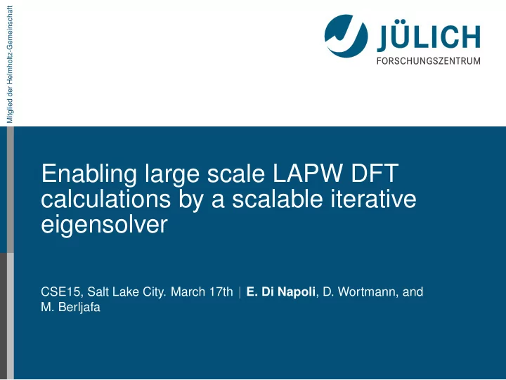
Mitglied der Helmholtz-Gemeinschaft Enabling large scale LAPW DFT calculations by a scalable iterative eigensolver CSE15, Salt Lake City. March 17th E. Di Napoli , D. Wortmann, and M. Berljafa

Typical Applications Atomic Structure Magnetic Electronic Structure Structure CSE15, Salt Lake City. March 17th E. Di Napoli , D. Wortmann, and M. Berljafa Folie 2

Outline The FLAPW method Sequences of correlated eigenproblems The algorithm: Chebyshev Accelerated Subspace Iteration (CHASE) CHASE parallelization and numerical tests CSE15, Salt Lake City. March 17th E. Di Napoli , D. Wortmann, and M. Berljafa Folie 3

Outline The FLAPW method Sequences of correlated eigenproblems The algorithm: Chebyshev Accelerated Subspace Iteration (CHASE) CHASE parallelization and numerical tests CSE15, Salt Lake City. March 17th E. Di Napoli , D. Wortmann, and M. Berljafa Folie 4

Density Functional Theory (DFT) 1 Φ ( x 1 ; s 1 , x 2 ; s 2 ,..., x n ; s n ) = ⇒ Λ i , a φ a ( x i ; s i ) 2 density of states n ( r ) = ∑ a f a | φ a ( r ) | 2 3 In the Schrödinger equation the exact Coulomb interaction is substituted with an effective potential V 0 ( r ) = V I ( r )+ V H ( r )+ V xc ( r ) Hohenberg-Kohn theorem ∃ one-to-one correspondence n ( r ) ↔ V 0 ( r ) = ⇒ V 0 ( r ) = V 0 ( r )[ n ] ∃ ! a functional E [ n ] : E 0 = min n E [ n ] The high-dimensional Schrödinger equation translates into a set of coupled non-linear low-dimensional self-consistent Kohn-Sham (KS) equation � � h 2 − ¯ 2 m ∇ 2 + V 0 ( r ) ˆ ∀ a H KS φ a ( r ) = φ a ( r ) = ε a φ a ( r ) solve CSE15, Salt Lake City. March 17th E. Di Napoli , D. Wortmann, and M. Berljafa Folie 5

DFT self-consistent field cycle Solve a set of Initial guess Compute discretized eigenproblems for charge density Kohn-Sham P ( ℓ ) k 1 ... P ( ℓ ) n start ( r ) equations k N No Compute new OUTPUT Converged? Yes charge density Electronic | n ( ℓ ) − n ( ℓ − 1 ) | < η structure, n ( ℓ ) ( r ) ... CSE15, Salt Lake City. March 17th E. Di Napoli , D. Wortmann, and M. Berljafa Folie 6

Zoo of methods LDA Plane waves GGA Localized basis set LDA + U Real space grids Hybrid functionals Green functions GW-approximation � � 2 m ∇ 2 + V 0 ( r ) h 2 − ¯ φ a ( r ) = ε a φ a ( r ) All-electron Finite differences Non-relaticistic eqs. Pseudo-potential Scalar-relativistic approx, Shape approximations Spin-orbit coupling Full-potential Dirac equation Spin polarized calculations CSE15, Salt Lake City. March 17th E. Di Napoli , D. Wortmann, and M. Berljafa Folie 7

Introduction to FLAPW LAPW basis set k Bloch vector ∑ c G ψ k , ν ( r ) = k , ν φ G ( k , r ) ν band index | G + k |≤ G max  e i ( k + G ) r Interstitial (I)  φ G ( k , r ) = � a α , G ℓ ( r )+ b α , G � ℓ m ( k ) u α u α ∑ ℓ m ( k ) ˙ ℓ ( r ) Y ℓ m ( ˆ r α ) Muffin Tin  ℓ, m boundary conditions Continuity of wavefunction and its derivative at MT boundary ⇓ a α , G b α , G ℓ m ( k ) and ℓ m ( k ) CSE15, Salt Lake City. March 17th E. Di Napoli , D. Wortmann, and M. Berljafa Folie 8

Where does the CPU time go? H and S Eigensolver Charge CPU time PE 50 % 13 % 33% 28 min. 1 27 % 20 % 44 % 36 min. 12 33 % 50 % 17 % 10 min. 30 23 % 61 % 11 % 12 min. 40 CSE15, Salt Lake City. March 17th E. Di Napoli , D. Wortmann, and M. Berljafa Folie 9

Where does the CPU time go? H and S Eigensolver Charge CPU time PE 50 % 13 % 33% 28 min. 1 27 % 20 % 44 % 36 min. 12 33 % 50 % 17 % 10 min. 30 23 % 61 % 11 % 12 min. 40 Solving the generalized eigenvalue problem 1 every P ( ℓ ) : A ( ℓ ) k c k = B ( ℓ ) k λ c k is a generalized eigenvalue problem; k 2 A and B are DENSE and hermitian (B is positive definite); 3 required: lower 2 ÷ 10 % of eigenpairs; 4 momentum vector index: k = 1 : 10 ÷ 100 ; 5 iteration cycle index: ℓ = 1 : 20 ÷ 50 . CSE15, Salt Lake City. March 17th E. Di Napoli , D. Wortmann, and M. Berljafa Folie 9

Outline The FLAPW method Sequences of correlated eigenproblems The algorithm: Chebyshev Accelerated Subspace Iteration (CHASE) CHASE parallelization and numerical tests CSE15, Salt Lake City. March 17th E. Di Napoli , D. Wortmann, and M. Berljafa Folie 10

Sequences of Eigenproblems Adjacent iteration cycles ITERATION ( ℓ ) ITERATION ( ℓ + 1 ) direct direct P ( ℓ ) ( X ( ℓ ) k 1 , Λ ( ℓ ) P ( ℓ + 1 ) ( X ( ℓ + 1 ) , Λ ( ℓ + 1 ) k 1 ) ) k 1 k 1 k 1 k 1 solver solver direct direct P ( ℓ ) ( X ( ℓ ) k 2 , Λ ( ℓ ) P ( ℓ + 1 ) ( X ( ℓ + 1 ) , Λ ( ℓ + 1 ) k 2 ) ) k 2 k 2 k 2 k 2 solver solver Next cycle direct direct P ( ℓ ) ( X ( ℓ ) k N , Λ ( ℓ ) P ( ℓ + 1 ) ( X ( ℓ + 1 ) , Λ ( ℓ + 1 ) k N ) ) k N k N k N k N solver solver X ≡ { x 1 ,..., x n } Λ ≡ diag ( λ 1 ,..., λ n ) CSE15, Salt Lake City. March 17th E. Di Napoli , D. Wortmann, and M. Berljafa Folie 11

Sequences of Eigenproblems Adjacent iteration cycles ITERATION ( ℓ ) ITERATION ( ℓ + 1 ) direct direct P ( ℓ ) ( X ( ℓ ) k 1 , Λ ( ℓ ) P ( ℓ + 1 ) ( X ( ℓ + 1 ) , Λ ( ℓ + 1 ) k 1 ) ) k 1 k 1 k 1 k 1 solver solver direct direct P ( ℓ ) ( X ( ℓ ) k 2 , Λ ( ℓ ) P ( ℓ + 1 ) ( X ( ℓ + 1 ) , Λ ( ℓ + 1 ) k 2 ) ) k 2 k 2 k 2 k 2 solver solver Next cycle direct direct P ( ℓ ) ( X ( ℓ ) k N , Λ ( ℓ ) P ( ℓ + 1 ) ( X ( ℓ + 1 ) , Λ ( ℓ + 1 ) k N ) ) k N k N k N k N solver solver X ≡ { x 1 ,..., x n } Λ ≡ diag ( λ 1 ,..., λ n ) CSE15, Salt Lake City. March 17th E. Di Napoli , D. Wortmann, and M. Berljafa Folie 11

Sequences of Eigenproblems Adjacent iteration cycles ITERATION ( ℓ ) ITERATION ( ℓ + 1 ) direct direct P ( ℓ ) ( X ( ℓ ) k 1 , Λ ( ℓ ) P ( ℓ + 1 ) ( X ( ℓ + 1 ) , Λ ( ℓ + 1 ) k 1 ) ) k 1 k 1 k 1 k 1 solver solver direct direct P ( ℓ ) ( X ( ℓ ) k 2 , Λ ( ℓ ) P ( ℓ + 1 ) ( X ( ℓ + 1 ) , Λ ( ℓ + 1 ) k 2 ) ) k 2 k 2 k 2 k 2 solver solver Next cycle direct direct P ( ℓ ) ( X ( ℓ ) k N , Λ ( ℓ ) P ( ℓ + 1 ) ( X ( ℓ + 1 ) , Λ ( ℓ + 1 ) k N ) ) k N k N k N k N solver solver X ≡ { x 1 ,..., x n } Λ ≡ diag ( λ 1 ,..., λ n ) CSE15, Salt Lake City. March 17th E. Di Napoli , D. Wortmann, and M. Berljafa Folie 11

Angles evolution An example Example: a metallic compound at fixed k Evolution of subspace angle for eigenvectors of k − point 1 and lowest 75 eigs 0 10 AuAg Angle b/w eigenvectors of adjacent iterations − 2 10 − 4 10 − 6 10 − 8 10 − 10 10 2 6 10 14 18 22 Iterations (2 − > 22) CSE15, Salt Lake City. March 17th E. Di Napoli , D. Wortmann, and M. Berljafa Folie 12

An alternative solving strategy Adjacent cycles ITERATION ( ℓ ) ITERATION ( ℓ + 1 ) iterative iterative P ( ℓ ) ( X ( ℓ ) k 1 , Λ ( ℓ ) P ( ℓ + 1 ) ( X ( ℓ + 1 ) , Λ ( ℓ + 1 ) k 1 ) ) k 1 k 1 k 1 k 1 solver solver iterative iterative P ( ℓ ) ( X ( ℓ ) k 2 , Λ ( ℓ ) P ( ℓ + 1 ) ( X ( ℓ + 1 ) , Λ ( ℓ + 1 ) k 2 ) ) k 2 k 2 k 2 k 2 solver solver Next cycle iterative iterative P ( ℓ ) ( X ( ℓ ) k N , Λ ( ℓ ) P ( ℓ + 1 ) ( X ( ℓ + 1 ) , Λ ( ℓ + 1 ) k N ) ) k N k N k N k N solver solver X ≡ { x 1 ,..., x n } Λ ≡ diag ( λ 1 ,..., λ n ) CSE15, Salt Lake City. March 17th E. Di Napoli , D. Wortmann, and M. Berljafa Folie 13

Outline The FLAPW method Sequences of correlated eigenproblems The algorithm: Chebyshev Accelerated Subspace Iteration (CHASE) CHASE parallelization and numerical tests CSE15, Salt Lake City. March 17th E. Di Napoli , D. Wortmann, and M. Berljafa Folie 14

Chebyshev Filtered Subspace Iteration method Properties and algorithm evolution Iterative solver musts input: the full set of multiple starting vectors Z 0 ≡ X ( ℓ − 1 ) ( : , 1 : NEV ) ; k i needed: it can efficiently use dense linear algebra kernels (i.e. xGEMM ); needed: it avoids stalling when facing small clusters of eigenvalues; Chebyshev Subspace Iteration Firstly introduced in [Rutishauser 1969] A version (called CheFSI) tailored to electronic structure computation in [Zhou, Saad, Tiago and Chelikowski 2006] for sparse eigenvalue problems. Our ChASE : 1) is tailored for dense eigenproblem sequences, 2) introduces a locking mechanism, 3) contains a refining inner loop, and 4) optimizes the polynomial degree. CSE15, Salt Lake City. March 17th E. Di Napoli , D. Wortmann, and M. Berljafa Folie 15

The core of the algorithm: Chebyshev filter Chebyshev polynomials A generic vector v = ∑ n i = 1 s i x i is very quickly aligned in the direction of the eigenvector corresponding to the extremal eigenvalue λ 1 n n v m = p m ( A ) v ∑ ∑ = s i p m ( A ) x i = s i p m ( λ i ) x i i = 1 i = 1 C m ( λ i − c n e ) ∑ = s 1 x 1 + x i ∼ s i s 1 x 1 C m ( λ 1 − c ) i = 2 e CSE15, Salt Lake City. March 17th E. Di Napoli , D. Wortmann, and M. Berljafa Folie 16

The core of the algorithm: Chebyshev filter In practice Three-terms recurrence relation C m + 1 ( t ) = 2 xC m ( t ) − C m − 1 ( t ) ; m ∈ N , C 0 ( t ) = 1 , C 1 ( t ) = x Z m . = p m ( ˜ ˜ H ) Z 0 with H = H − cI n F OR : i = 1 → DEG − 1 Z i + 1 ← 2 σ i + 1 ˜ H × Z i − σ i + 1 σ i Z i − 1 xGEMM e E ND F OR . CSE15, Salt Lake City. March 17th E. Di Napoli , D. Wortmann, and M. Berljafa Folie 17