Empirically Comparing the Finite-Time Performance of - PowerPoint PPT Presentation
Empirically Comparing the Finite-Time Performance of Simulation-Optimization Algorithms Anna Dong, David Eckman , Xueqi Zhao, Shane Henderson Cornell University Matthias Poloczek University of Arizona Winter Simulation Conference December 5,
Empirically Comparing the Finite-Time Performance of Simulation-Optimization Algorithms Anna Dong, David Eckman , Xueqi Zhao, Shane Henderson Cornell University Matthias Poloczek University of Arizona Winter Simulation Conference December 5, 2017
C OMPARING S IMULATION -O PTIMIZATION A LGORITHMS D ONG ET AL . Simulation Optimization (SO) Optimize a real-valued objective function, estimated via simulation, over a deterministic domain. Challenges: 1. Error in estimating objective function. 2. Unknown topology (continuity/differentiability/convexity). SO algorithms are designed to solve a broad class of problems. I NTRODUCTION E VALUATION E XPERIMENTS P LOTS C ONCLUSIONS 2/22
C OMPARING S IMULATION -O PTIMIZATION A LGORITHMS D ONG ET AL . SO Algorithm Performance Many theoretical results for asymptotic performance, • . . . as simulation budget approaches infinity. Examples: • Algorithm converges to local (global) optimizer. • Convergence rate, once within neighborhood of optimizer. Required budget for such results may exceed practical budget! To decide which algorithm to use, a practitioner cares about finite-time performance. I NTRODUCTION E VALUATION E XPERIMENTS P LOTS C ONCLUSIONS 3/22
C OMPARING S IMULATION -O PTIMIZATION A LGORITHMS D ONG ET AL . Evaluating Algorithms SO community lags behind other optimization communities: • Established testbed of problems for benchmarking. • Metrics for empirical finite-time performance. • Comparison of algorithms on large testbed. We implement several popular SO algorithms and test them on a subset of problems from the SimOpt library ✭✇✇✇✳s✐♠♦♣t✳♦r❣✮ . I NTRODUCTION E VALUATION E XPERIMENTS P LOTS C ONCLUSIONS 4/22
C OMPARING S IMULATION -O PTIMIZATION A LGORITHMS D ONG ET AL . Objectives Near-term: 1. Comparison of finite-time performance of different algorithms. 2. Insights on the types of problems on which certain algorithms work well. Long-term: 1. More contributions to SimOpt library. • Problems and/or algorithms. 2. Development of finite-time performance metrics. • E.g., adapting performance profiles. 3. Motivate others to do similar comparisons. 4. Development of algorithms with strong finite-time performance. I NTRODUCTION E VALUATION E XPERIMENTS P LOTS C ONCLUSIONS 5/22
C OMPARING S IMULATION -O PTIMIZATION A LGORITHMS D ONG ET AL . Evaluating Finite-Time Performance In deterministic optimization: • Measure computational effort needed to get to optimal solution (or within specified tolerance). • Number of function evaluations or wall clock time. Doesn’t work so well for SO. • Optimal solution is often unknown. • Often no certificate of optimality. • Estimation error makes it hard to check tolerance condition. I NTRODUCTION E VALUATION E XPERIMENTS P LOTS C ONCLUSIONS 6/22
C OMPARING S IMULATION -O PTIMIZATION A LGORITHMS D ONG ET AL . Evaluating Finite-Time Performance Idea 1. Fix a simulation budget. 2. Evaluate the objective function at the estimated best solution found within the budget. We measure the budget in number of objective function evaluations. I NTRODUCTION E VALUATION E XPERIMENTS P LOTS C ONCLUSIONS 7/22
C OMPARING S IMULATION -O PTIMIZATION A LGORITHMS D ONG ET AL . Evaluating Finite-Time Performance Let Z ( n ) be the true objective function value of the estimated best solution visited in the first n objective function evaluations. • Z ( n ) is a random variable, because the estimated best solution, X ( n ) , is random. • Conditional on X ( n ) , Z ( n ) is fixed, but needs to be estimated. In our experiments, we estimate Z ( n ) (conditional on X ( n ) ) in a post-processing step. I NTRODUCTION E VALUATION E XPERIMENTS P LOTS C ONCLUSIONS 8/22
C OMPARING S IMULATION -O PTIMIZATION A LGORITHMS D ONG ET AL . Evaluating Finite-Time Performance Figure: Pasupathy and Henderson (2006). I NTRODUCTION E VALUATION E XPERIMENTS P LOTS C ONCLUSIONS 9/22
C OMPARING S IMULATION -O PTIMIZATION A LGORITHMS D ONG ET AL . Evaluating Finite-Time Performance Can obtain Z ( n ) curve from single macroreplication of an algorithm. • Unless the algorithm uses the budget in setting parameters. Location of Z ( n ) curve is random, so take several macroreplications and look at: • mean, • median/quantile, • empirical cdf (hard to show on one plot) . I NTRODUCTION E VALUATION E XPERIMENTS P LOTS C ONCLUSIONS 10/22
C OMPARING S IMULATION -O PTIMIZATION A LGORITHMS D ONG ET AL . Algorithms 1. Random Search (non-adaptive) 2. Gradient Search with Random Restarts • Central finite differences for gradient estimate. 3. Simultaneous Perturbation Stochastic Approximation (SPSA) • Uses budget to set gain sequence. 4. Stochastic Trust-Region Response-Surface Method (STRONG) • Didn’t use design of experiments for fitting. • Central finite differences for gradient estimate. a. BFGS estimate of Hessian. (STRONG) b. No second-order model. (STRONG-Stage1) 5. Nelder-Mead • Simplicial method that doesn’t use gradient information. I NTRODUCTION E VALUATION E XPERIMENTS P LOTS C ONCLUSIONS 11/22
C OMPARING S IMULATION -O PTIMIZATION A LGORITHMS D ONG ET AL . Benchmark Problems Table: SimOpt benchmark problems and their characteristics. Name on SimOpt Dimension Optimal Solution A Multimodal Function 2 Known Ambulances in a Square 6 Unknown Continuous Newsvendor 1 Known Dual Sourcing 2 Unknown Economic-Order-Quantity 1 Known Facility Location 4 Unknown GI/G/1 Queue 1 Unknown M/M/1 Metamodel 3 Known Optimal Controller for a POMDP 10 Unknown Optimization of a Production Line 3 Unknown Parameter Estimation: 2D Gamma 2 Known Rosenbrock’s Function 40 Known Route Prices for Mobility-on-Demand 12 Unknown SAN Duration 13 Unknown Toll Road Improvements 12 Unknown I NTRODUCTION E VALUATION E XPERIMENTS P LOTS C ONCLUSIONS 12/22
C OMPARING S IMULATION -O PTIMIZATION A LGORITHMS D ONG ET AL . Problems Properties of all problems: • Continuous decision variables. • Deterministic (box) constraints or unbounded. Initial solution is drawn from probability distribution over domain. • Uniform distribution for bounded variables. • Exponential/Laplace distribution for unbounded variables. Took 30 replications at given solution to estimate its objective value. • Used common random numbers (CRN) across solutions. I NTRODUCTION E VALUATION E XPERIMENTS P LOTS C ONCLUSIONS 13/22
C OMPARING S IMULATION -O PTIMIZATION A LGORITHMS D ONG ET AL . Experiments For every problem: • Ran 30 macroreplications of each algorithm. • Recorded estimated best solution X ( n ) for range of n values. • Ran 30 function evaluations at each X ( n ) to estimate Z ( n ) conditional on X ( n ) . • Averaged 30 estimates of Z ( n ) . • Constructed 95% normal confidence intervals. I NTRODUCTION E VALUATION E XPERIMENTS P LOTS C ONCLUSIONS 14/22
C OMPARING S IMULATION -O PTIMIZATION A LGORITHMS D ONG ET AL . Rosenbrock ( dim = 40 ) # 10 6 minimize Problem: Rosenbrock 4.5 Random Search 4 Nelder-Mead Gradient Search RS 3.5 SPSA Objective value STRONG 3 STRONG-StageI 2.5 2 1.5 1 0.5 0 2 4 6 8 10 12 Budget # 10 4 I NTRODUCTION E VALUATION E XPERIMENTS P LOTS C ONCLUSIONS 15/22
C OMPARING S IMULATION -O PTIMIZATION A LGORITHMS D ONG ET AL . Facility Location ( dim = 4 ) maximize Problem: FacilityLocation 0.35 0.3 Objective value 0.25 Random Search Nelder-Mead Gradient Search RS 0.2 SPSA STRONG STRONG-StageI 0.15 0 0.5 1 1.5 2 2.5 3 Budget # 10 4 I NTRODUCTION E VALUATION E XPERIMENTS P LOTS C ONCLUSIONS 16/22
C OMPARING S IMULATION -O PTIMIZATION A LGORITHMS D ONG ET AL . Ambulance ( dim = 6 ) minimize Problem: Ambulance 0.2 Random Search 0.19 Nelder-Mead Gradient Search RS SPSA Objective value 0.18 STRONG STRONG-StageI 0.17 0.16 0.15 0.14 0 0.5 1 1.5 2 2.5 3 Budget # 10 4 I NTRODUCTION E VALUATION E XPERIMENTS P LOTS C ONCLUSIONS 17/22
C OMPARING S IMULATION -O PTIMIZATION A LGORITHMS D ONG ET AL . Route Prices ( dim = 12 ) maximize Problem: RoutePrices 1300 1200 1100 Objective value 1000 900 Random Search Nelder-Mead 800 Gradient Search RS SPSA 700 STRONG STRONG-StageI 600 0 1 2 3 4 5 Budget # 10 4 I NTRODUCTION E VALUATION E XPERIMENTS P LOTS C ONCLUSIONS 18/22
C OMPARING S IMULATION -O PTIMIZATION A LGORITHMS D ONG ET AL . Stochastic Activity Network ( dim = 13 ) minimize Problem: SAN 26 Random Search 25 Nelder-Mead Gradient Search RS 24 SPSA Objective value STRONG STRONG-StageI 23 22 21 20 19 0 2 4 6 8 10 Budget # 10 4 I NTRODUCTION E VALUATION E XPERIMENTS P LOTS C ONCLUSIONS 19/22
C OMPARING S IMULATION -O PTIMIZATION A LGORITHMS D ONG ET AL . POMDP Controller ( dim = 10 ) minimize Problem: POMDPController 143 Random Search Nelder-Mead Gradient Search RS 142 SPSA Objective value STRONG 141 STRONG-StageI 140 139 138 137 136 0 0.5 1 1.5 2 2.5 3 # 10 4 Budget I NTRODUCTION E VALUATION E XPERIMENTS P LOTS C ONCLUSIONS 20/22
C OMPARING S IMULATION -O PTIMIZATION A LGORITHMS D ONG ET AL . Conclusions Takeaways 1. Robust performance of Nelder-Mead across problems. 2. STRONG-Stage1 did as well as (or better than) STRONG. 3. Random Search did better than expected. 4. Performance of SPSA was sometimes highly variable. I NTRODUCTION E VALUATION E XPERIMENTS P LOTS C ONCLUSIONS 21/22
Recommend
More recommend
Explore More Topics
Stay informed with curated content and fresh updates.
