Empirical Process Theory for Statistics Jon A. Wellner University - PowerPoint PPT Presentation

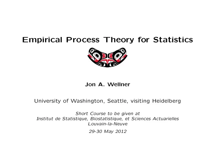
Empirical Process Theory for Statistics Jon A. Wellner University of Washington, Seattle, visiting Heidelberg Short Course to be given at Institut de Statistique, Biostatistique, et Sciences Actuarielles Louvain-la-Neuve 29-30 May 2012

Short Course, Louvain-la-Neuve • Day 1 (Tuesday): ⊲ Lecture 1: Introduction, history, selected examples. ⊲ Lecture 2: Some basic inequalities and Glivenko-Cantelli theorems. ⊲ Lecture 3: Using the Glivenko-Cantelli theorems: first applications. Based on Courses given at Torgnon, Cortona, and Delft (2003-2005). Notes available at: http://www.stat.washington.edu/jaw/ RESEARCH/TALKS/talks.html Short Course, Louvain-la-Neuve; 29-30 May 2012 1.1

• Day 2 (Wednesday): ⊲ Donsker theorems and some inequalities ⊲ Peeling methods and rates of convergence ⊲ Some useful preservation theorems. Short Course, Louvain-la-Neuve; 29-30 May 2012 1.2

Lecture 1: Introduction, history, selected examples • 1. Classical empirical processes • 2. Modern empirical processes • 3. Some examples Short Course, Louvain-la-Neuve; 29-30 May 2012 1.3

1. Classical empirical processes. Suppose that: • X 1 , . . . , X n are i.i.d. with d.f. F on R . • F n ( x ) = n − 1 � n i =1 1 [ X i ≤ x ] , the empirical distribution function. • { Z n ( x ) ≡ √ n ( F n ( x ) − F ( x )) : x ∈ R } , the empirical process. Two classical theorems: Theorem 1. (Glivenko-Cantelli, 1933). � F n − F � ∞ ≡ −∞ <x< ∞ | F n ( x ) − F ( x ) | → a.s. 0 . sup Theorem 2. (Donsker, 1952). Z n ⇒ Z ≡ U ( F ) in D ( R, � · � ∞ ) Short Course, Louvain-la-Neuve; 29-30 May 2012 1.4

where U is a standard Brownian bridge process on [0 , 1]; i.e. U is a zero-mean Gaussian process with covariance E ( U ( s ) U ( t )) = s ∧ t − st, s, t ∈ [0 , 1] . This means that we have Eg ( Z n ) → Eg ( Z ) for any bounded, continuous function g : D ( R , � · � ∞ ) → R and g ( Z n ) → d g ( Z ) for any continuous function g : D ( R , � · � ∞ ) → R (ignoring measurability issues). Short Course, Louvain-la-Neuve; 29-30 May 2012 1.5

2. General empirical processes (indexed by functions) Suppose that: • X 1 , . . . , X n are i.i.d. with probability measure P on ( X , A ). • P n = n − 1 � n i =1 δ X i , the empirical measure; here � 1 , x ∈ A, δ x ( A ) = 1 A ( x ) = for A ∈ A . x ∈ A c 0 , Hence we have n n � � P n ( A ) = n − 1 P n ( f ) = n − 1 1 A ( X i ) , and f ( X i ) . i =1 i =1 • { G n ( f ) ≡ √ n ( P n ( f ) − P ( f )) : f ∈ F ⊂ L 2 ( P ) } , the empirical process indexed by F Short Course, Louvain-la-Neuve; 29-30 May 2012 1.6

Note that the classical case corresponds to: • ( X , A ) = ( R , B ). • F = { 1 ( −∞ ,t ] ( · ) : t ∈ R } . Then n � P n (1 ( −∞ ,t ] ) = n − 1 1 ( −∞ ,t ] ( X i ) = F n ( t ) , i =1 P (1 ( −∞ ,t ] ) = F ( t ) , G n (1 ( −∞ ,t ] ) = √ n ( P n − P )(1 ( −∞ ,t ] = √ n ( F n ( t ) − F ( t )) G (1 ( −∞ ,t ] ) = U ( F ( t )) . Short Course, Louvain-la-Neuve; 29-30 May 2012 1.7

Two central questions for the general theory: A. For what classes of functions F does a natural generalization of the Glivenko-Cantelli theorem hold? That is, for what classes F do we have � P n − P � ∗ F → a.s. 0 If this convergence holds, then we say that F is a P − Glivenko- Cantelli class of functions. B. For what classes of functions F does a natural generalization of Donsker’s theorem hold? That is, for what classes F do we have ℓ ∞ ( F )? G n ⇒ G in If this convergence holds, then we say that F is a P − Donsker class of functions. Short Course, Louvain-la-Neuve; 29-30 May 2012 1.8

Here G is a 0 − mean P − Brownian bridge process with uniformly- continuous sample paths with respect to the semi-metric ρ P ( f, g ) defined by ρ 2 P ( f, g ) = V ar P ( f ( X ) − g ( X )) , ℓ ∞ ( F ) is the space of all bounded, real-valued functions from F to R : � � � � � ℓ ∞ ( F ) = x : F �→ R � � x � F ≡ sup | x ( f ) | < ∞ , � f ∈F and E { G ( f ) G ( g ) } = P ( fg ) − P ( f ) P ( g ) . Short Course, Louvain-la-Neuve; 29-30 May 2012 1.9

3. Some Examples A commonly occurring problem in statistics: we want to prove consistency or asymptotic normality of some statistic which is not a sum of independent random variables, but which can be related to some natural sum of random functions indexed by a parameter in a suitable (metric) space. Example 1. Suppose that X 1 , . . . , X n are i.i.d. real-valued with E | X 1 | < ∞ , and let µ = E ( X 1 ). Consider the absolute deviations about the sample mean, n � D n = P n | X − X n | = n − 1 | X i − X n | . i =1 Since X n → a.s. µ , we know that for any δ > 0 we have X ∈ [ µ − δ, µ + δ ] for all sufficiently large n almost surely. Thus we see that if we define n � D n ( t ) ≡ n − 1 P n | x − t | = n − 1 | X i − t | , i =1 Short Course, Louvain-la-Neuve; 29-30 May 2012 1.10

then D n = D n ( X n ) and study of D n ( t ) for t ∈ [ µ − δ, µ + δ ] is equivalent to study of the empirical measure P n indexed by the class of functions F δ = { x �→ | x − t | ≡ f t ( x ) : t ∈ [ µ − δ, µ + δ ] } . To show that D n → a.s. d ≡ E | X − µ | , we write D n − d = P n | X − X n | − P | X − µ | (1) = ( P n − P )( | X − X n | ) + P | X − X n | − P | X − µ | ≡ I n + II n . (2) Now | I n | = | ( P n − P )( | X − X n | ) | ≤ sup | ( P n − P ) | X − t || = sup | ( P n − P )( f ) | f ∈F δ t : | t − µ |≤ δ → a.s. 0 (3) if F δ is P − Glivenko-Cantelli. Short Course, Louvain-la-Neuve; 29-30 May 2012 1.11

But convergence of the second term in (2) is easy: by the triangle inequality II n = | P | X − X n | − P | X − µ || ≤ P | X n − µ | = | X n − µ | → a.s. 0 . How to prove (3)? Consider the functions f 1 , . . . , f m ∈ F δ given by f j ( x ) = | x − ( µ − δ (1 − j/m ) | , j = 0 , . . . , 2 m. For this finite set of functions we have 0 ≤ j ≤ 2 m | ( P n − P )( f j ) | → a.s. 0 max by the strong law of large numbers applied 2 m + 1 times. Furthermore ... Short Course, Louvain-la-Neuve; 29-30 May 2012 1.12

it follows that for t ∈ [ µ − δ (1 − j/m ) , µ − δ (1 − ( j + 1) /m )] the functions f t ( x ) = | x − t | satisfy (picture!) L j ( x ) ≡ f j/m ( x ) ∧ f ( j +1) /m ( x ) ≤ f t ( x ) ≤ f j/m ( x ) ∨ f ( j +1) /m ( x ) ≡ U j ( x ) where U j ( x ) − f t ( x ) ≤ 1 f t ( x ) − L j ( x ) ≤ 1 U j ( x ) − L j ( x ) ≤ 1 m, m, m. Thus for each m � P n − P � F δ ≡ sup | ( P n − P )( f ) | f ∈F δ � � ≤ max 0 ≤ j ≤ 2 m | ( P n − P )( U j ) | , max 0 ≤ j ≤ 2 m | ( P n − P )( L j ) | max + 1 /m → a.s. 0 + 1 /m Taking m large shows that (3) holds. Short Course, Louvain-la-Neuve; 29-30 May 2012 1.13

This is a bracketing argument, and generalizes easily to yield a quite general bracketing Glivenko-Cantelli theorem. How to prove √ n ( D n − d ) → d ? We write √ n ( D n − d ) √ n ( P n | X − X n | − P | X − µ | ) = √ n ( P n | X − µ | − P | X − µ | ) = + √ n ( P | X − X n | − P | X − µ | ) + √ n ( P n − P )( | X − X n | ) − √ n ( P n − P )( | X − µ | ) G n ( | X − µ | ) + √ n ( H ( X n ) − H ( µ )) = + G n ( | X − X n | − | X − µ | ) G n ( | X − µ | ) + H ′ ( µ )( X n − µ ) = + √ n ( H ( X n ) − H ( µ ) − H ′ ( µ )( X n − µ )) + G n ( | X − X n | − | X − µ | ) G n ( | X − µ | + H ′ ( µ )( X − µ )) + I n + II n ≡ where ... Short Course, Louvain-la-Neuve; 29-30 May 2012 1.14

H ( t ) ≡ P | X − t | , √ n ( H ( X n ) − H ( µ ) − H ′ ( µ )( X n − µ )) , I n ≡ II n ≡ G n ( | X − X n | ) − G n ( | X − µ | ) = G n ( | X − X n | − | X − µ | ) = G n ( f X n − f µ ) . Here I n → p 0 if H ( t ) ≡ P | X − t | is differentiable at µ , and II n → p 0 if F δ is a Donsker class of functions! This is a consequence of asymptotic equicontinuity of G n over the class F : for every ǫ > 0 n →∞ Pr ∗ ( δ ց 0 lim sup lim sup | G n ( f ) − G n ( g ) | > ǫ ) = 0 . f,g : ρ P ( f,g ) ≤ δ Short Course, Louvain-la-Neuve; 29-30 May 2012 1.15

Example 2. Copula models: the pseudo-MLE. Let c θ ( u 1 , . . . , u p ) be a copula density with θ ⊂ Θ ⊂ R q . Suppose that X 1 , . . . , X n are i.i.d. with density f ( x 1 , . . . , x p ) = c θ ( F 1 ( x 1 ) , . . . , F p ( x p )) · f 1 ( x 1 ) · · · f p ( x p ) where F 1 , . . . , F p are absolutely continuous d.f.’s with densities f 1 , . . . , f p . Let n � F n,j ( x j ) ≡ n − 1 1 { X i,j ≤ x j } , j = 1 , . . . , p i =1 be the marginal empirical d.f.’s of the data. Then a natural pseudo-likelihood function is given by l n ( θ ) ≡ P n log c θ ( F n, 1 ( x 1 ) , . . . , F n,p ( x p )) . Short Course, Louvain-la-Neuve; 29-30 May 2012 1.16

Thus it seems reasonable to define the pseudo-likelihood esti- mator � θ n of θ by the q − dimensional system of equations Ψ n ( � θ n ) = 0 where Ψ n ( θ ) ≡ P n ( ˙ ℓ θ ( θ ; F n, 1 ( x 1 ) , . . . , F n,p ( x p )) and where ˙ ℓ θ ( θ ; u 1 , . . . , u p ) ≡ ∇ θ log c θ ( u 1 , . . . , u p ) . We also define Ψ( θ ) by Ψ( θ ) ≡ P 0 ( ˙ ℓ θ ( θ, F 1 ( x 1 ) , . . . , F p ( x p )) . Short Course, Louvain-la-Neuve; 29-30 May 2012 1.17