Eliminating the Invariance on the Loss Landscape of Linear - PowerPoint PPT Presentation

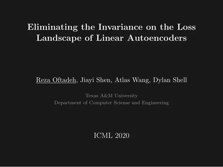
Eliminating the Invariance on the Loss Landscape of Linear Autoencoders Reza Oftadeh, Jiayi Shen, Atlas Wang, Dylan Shell Texas A&M University Department of Computer Sciense and Engineering ICML 2020

Overview ◮ Linear Autoencoder (LAE) with Mean Square Error (MSE). The classical results: – Loss surface has been analytically characterized. – All local minima are global minima. – The columns of the optimal decoder does not identify the principal directions but only their low dimensional subspace (the so-called invariance problem). ◮ We present a new loss function for LAE: – Analytically characterize the loss landscape. – All local minima are global minima. – The columns of the optimal decoder span the principal directions . – Invariant local minima become saddle points. – Computational complexity is of the same order of MSE loss. 2

Overview ◮ Linear Autoencoder (LAE) with Mean Square Error (MSE). The classical results: – Loss surface has been analytically characterized. – All local minima are global minima. – The columns of the optimal decoder does not identify the principal directions but only their low dimensional subspace (the so-called invariance problem). ◮ We present a new loss function for LAE: – Analytically characterize the loss landscape. – All local minima are global minima. – The columns of the optimal decoder span the principal directions . – Invariant local minima become saddle points. – Computational complexity is of the same order of MSE loss. 2

Overview ◮ Linear Autoencoder (LAE) with Mean Square Error (MSE). The classical results: – Loss surface has been analytically characterized. – All local minima are global minima. – The columns of the optimal decoder does not identify the principal directions but only their low dimensional subspace (the so-called invariance problem). ◮ We present a new loss function for LAE: – Analytically characterize the loss landscape. – All local minima are global minima. – The columns of the optimal decoder span the principal directions . – Invariant local minima become saddle points. – Computational complexity is of the same order of MSE loss. 2

Overview ◮ Linear Autoencoder (LAE) with Mean Square Error (MSE). The classical results: – Loss surface has been analytically characterized. – All local minima are global minima. – The columns of the optimal decoder does not identify the principal directions but only their low dimensional subspace (the so-called invariance problem). ◮ We present a new loss function for LAE: – Analytically characterize the loss landscape. – All local minima are global minima. – The columns of the optimal decoder span the principal directions . – Invariant local minima become saddle points. – Computational complexity is of the same order of MSE loss. 2

Overview ◮ Linear Autoencoder (LAE) with Mean Square Error (MSE). The classical results: – Loss surface has been analytically characterized. – All local minima are global minima. – The columns of the optimal decoder does not identify the principal directions but only their low dimensional subspace (the so-called invariance problem). ◮ We present a new loss function for LAE: – Analytically characterize the loss landscape. – All local minima are global minima. – The columns of the optimal decoder span the principal directions . – Invariant local minima become saddle points. – Computational complexity is of the same order of MSE loss. 2

Overview ◮ Linear Autoencoder (LAE) with Mean Square Error (MSE). The classical results: – Loss surface has been analytically characterized. – All local minima are global minima. – The columns of the optimal decoder does not identify the principal directions but only their low dimensional subspace (the so-called invariance problem). ◮ We present a new loss function for LAE: – Analytically characterize the loss landscape. – All local minima are global minima. – The columns of the optimal decoder span the principal directions . – Invariant local minima become saddle points. – Computational complexity is of the same order of MSE loss. 2

Overview ◮ Linear Autoencoder (LAE) with Mean Square Error (MSE). The classical results: – Loss surface has been analytically characterized. – All local minima are global minima. – The columns of the optimal decoder does not identify the principal directions but only their low dimensional subspace (the so-called invariance problem). ◮ We present a new loss function for LAE: – Analytically characterize the loss landscape. – All local minima are global minima. – The columns of the optimal decoder span the principal directions . – Invariant local minima become saddle points. – Computational complexity is of the same order of MSE loss. 2

Overview ◮ Linear Autoencoder (LAE) with Mean Square Error (MSE). The classical results: – Loss surface has been analytically characterized. – All local minima are global minima. – The columns of the optimal decoder does not identify the principal directions but only their low dimensional subspace (the so-called invariance problem). ◮ We present a new loss function for LAE: – Analytically characterize the loss landscape. – All local minima are global minima. – The columns of the optimal decoder span the principal directions . – Invariant local minima become saddle points. – Computational complexity is of the same order of MSE loss. 2

Overview ◮ Linear Autoencoder (LAE) with Mean Square Error (MSE). The classical results: – Loss surface has been analytically characterized. – All local minima are global minima. – The columns of the optimal decoder does not identify the principal directions but only their low dimensional subspace (the so-called invariance problem). ◮ We present a new loss function for LAE: – Analytically characterize the loss landscape. – All local minima are global minima. – The columns of the optimal decoder span the principal directions . – Invariant local minima become saddle points. – Computational complexity is of the same order of MSE loss. 2

Overview ◮ Linear Autoencoder (LAE) with Mean Square Error (MSE). The classical results: – Loss surface has been analytically characterized. – All local minima are global minima. – The columns of the optimal decoder does not identify the principal directions but only their low dimensional subspace (the so-called invariance problem). ◮ We present a new loss function for LAE: – Analytically characterize the loss landscape. – All local minima are global minima. – The columns of the optimal decoder span the principal directions . – Invariant local minima become saddle points. – Computational complexity is of the same order of MSE loss. 2

Setup ◮ Data: m sample points of dimension n : – Input: x j ∈ R n , Output: y j ∈ R n for j = 1 , . . . , m . – In matrix form: X ∈ R n × m , Y ∈ R n × m . ◮ LAE: A neural network with linear activation functions and single hidden layer of width p < n . x j ∈ R n y j ∈ R n B ∈ R p × n A ∈ R n × p Encoder Decoder ˆ p < n – The weights: The encoder matrix B , and the decoder matrix A . y j = ABx j or ˆ – The global map is ˆ Y = ABX . 3

Setup ◮ Data: m sample points of dimension n : – Input: x j ∈ R n , Output: y j ∈ R n for j = 1 , . . . , m . – In matrix form: X ∈ R n × m , Y ∈ R n × m . ◮ LAE: A neural network with linear activation functions and single hidden layer of width p < n . x j ∈ R n y j ∈ R n B ∈ R p × n A ∈ R n × p Encoder Decoder ˆ p < n – The weights: The encoder matrix B , and the decoder matrix A . y j = ABx j or ˆ – The global map is ˆ Y = ABX . 3

Setup ◮ Data: m sample points of dimension n : – Input: x j ∈ R n , Output: y j ∈ R n for j = 1 , . . . , m . – In matrix form: X ∈ R n × m , Y ∈ R n × m . ◮ LAE: A neural network with linear activation functions and single hidden layer of width p < n . x j ∈ R n y j ∈ R n B ∈ R p × n A ∈ R n × p Encoder Decoder ˆ p < n – The weights: The encoder matrix B , and the decoder matrix A . y j = ABx j or ˆ – The global map is ˆ Y = ABX . 3

Setup ◮ Data: m sample points of dimension n : – Input: x j ∈ R n , Output: y j ∈ R n for j = 1 , . . . , m . – In matrix form: X ∈ R n × m , Y ∈ R n × m . ◮ LAE: A neural network with linear activation functions and single hidden layer of width p < n . x j ∈ R n y j ∈ R n B ∈ R p × n A ∈ R n × p Encoder Decoder ˆ p < n – The weights: The encoder matrix B , and the decoder matrix A . y j = ABx j or ˆ – The global map is ˆ Y = ABX . 3

Setup ◮ Data: m sample points of dimension n : – Input: x j ∈ R n , Output: y j ∈ R n for j = 1 , . . . , m . – In matrix form: X ∈ R n × m , Y ∈ R n × m . ◮ LAE: A neural network with linear activation functions and single hidden layer of width p < n . x j ∈ R n y j ∈ R n B ∈ R p × n A ∈ R n × p Encoder Decoder ˆ p < n – The weights: The encoder matrix B , and the decoder matrix A . y j = ABx j or ˆ – The global map is ˆ Y = ABX . 3