Electric Spot Prices and Wind Forecasts: A dynamic Nordic/Baltic - PowerPoint PPT Presentation

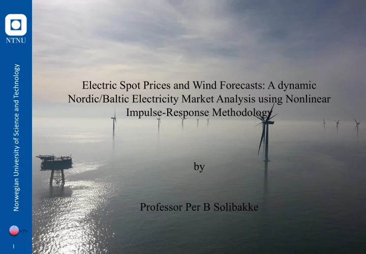
Norwegian University of Science and Technology Electric Spot Prices and Wind Forecasts: A dynamic Nordic/Baltic Electricity Market Analysis using Nonlinear Impulse-Response Methodology by Professor Per B Solibakke 4.2% 1 1

Spot Electricity Prices and Wind Forecasts. Dynamic Impulse-Response Analysis Introduction  A dynamic daily market approach is established from the Nordic/Baltic Electricity market (NordPool). The period with available data wind forecasts is from January 2013 to May 2017. The daily wind information in MWh is shown below: 8.3% 2 2

Spot Electricity Prices and Wind Forecasts. Dynamic Impulse-Response Analysis Introduction  The daily electricity price information in MWh for the Nordic/Baltic Electricity market (NordPool) 2013-2017 is shown below: 12.5% 3 3

Spot Electricity Prices and Wind Forecasts. Dynamic Impulse-Response Analysis The Impulse-Response Methodology Impulse Responses for the Mean Equation: The paper applies the methodologies outlined by Gallant et al. (1993) defining one-step ahead forecast for the mean conditioned on the history as (for a Markovian process) ( y = spot price and wind forecast changes):       L- 1 g y ,...,y =E y | y t- L+ 1 t t+ 1 t- k k= 0       =E g y ,...,y | x =x y x t- L+j t+j t i j for i = - 60,…,60 and j = 0,…,5, where We write: and therefore y     j =E E y | y ,...,y | x =x   x = y ,...,y t+j t- L+j t+j t L+ - 1 0   ∞ -10 y Note that represent the response to a negative 10% impulse. Here the responses depend upon the initial change x , which reflects j j the non-linearity.   , ∞ i 0 y - y    We report , which represents the effects of the shocks on the trajectories of the process itself. i 60,...,60 and j 0,...,5 j j j     L=1     E g y ,..., y | y , j = 0,1,...,5 , A conditional profile can therefore be defined as:  t+ j-J t+ j t-k  k=0 16.7% 4 4

Spot Electricity Prices and Wind Forecasts. Dynamic Impulse-Response Analysis The Impulse-Response Methodology Impulse Responses for the Variance Equation: Defining one-step ahead variance (volatility), is the on-step ahead forecast for the variance conditioned on the history as ( y = spot price and wind forecast changes):        ′              ∞ ∞ ∞ ∞ Var y | y =E y E y - y x y - E y | y | y       t+ 1 t- k  t+ 1 t+ 1 t- k   t+ 1 t+ 1 t- k  t- k k= 0 k= 0 k= 0 k= 0         x = E g y ,..., y | x = x ψ j t-L+ j t+ j t   x = y ,...,y for j = 0,…,5, where We write:     L+ - 1 0 = E Var y | x | x = x t+ j t+ j-1 t   ∞ -10  Note that represent the volatility response to a negative 10% impulse. The responses depend upon the initial change x . j j   , ∞ i 0 -      i 60,...,60 and j 0,...,5 We report , which represents the effects of the shocks on the trajectories of the process itself. j j j The conditional volatility profile is different from the path described by the j -step ahead square error process. Note that analytical evaluation of the integrals in the definition of a conditional moment profile is intractable. However, evaluation is well suited to Monte Carlo integration. For simulated realisations we write (with approximation error tending to zero almost surely as R → ∞):  j- 1           g x = ... g y ,...,y f y | y ,...,y dy ...dy   j j- J j i+ 1 y- L+ 1 i 1 j   i=0 R      1 / R g y r ,...,y r j j- J r= 1 20.8% 5 5 Sup-norm bands (confidence intervals) are constructed by bootstrapping (changing seed generates densities and impulse response samples)

Spot Electricity Prices and Wind Forecasts. Dynamic Impulse-Response Analysis Literature review Spot Electricity Prices: Goto and Karolyi (2004), Chan and Gray (2006), Theodorou and Karyampas (2008), Bystrøm (2003) and Solibakke (2002). Higgs and Worthington (2008), Huisman and Mahieu ((2003) and Thomas et al., (2011). De Vany and Walls (1999), Higgs and Worthington (2008), Huisman and Mahieu (2003), Huisman and Kilic (2013), Haldrup and Nilsen (2006), Knittel (2005), Li and Flynn (2004), Lindstrom and Regland (2012), Mount, Ning and Cai (2006), Robinson (2000), Robinson and Baniak (2002), Rubin and Babcock (2011), Tashpulatov (2013), and Weron (2006, 2008). Chan and Gray (2006), Escribano, Pena and Villaplana (2011), Habell, Marathe and Shawky (2004), Higgs and Worthington (2005), Koopman, Ooms and Carnero (2007) and Solibakke (2002). Weron (2006, 2008), Harris (2006), Geman and Roncoroni (2006), Koopman et al. (2007) and Pilipovic (2007). Wind Forecasts: Price changes: Skytte, 1999, Morthorst, 2003 , Giabardo et al., 2009, and Traber and Kenfert, 2011 Price Volatility: Green and Vasilakos (2010), Steggals et al. (2011), Woo et al. (2011), Jacobsen and Zvingilaite (2010), and Twomey and Neuhoff (2010), The Semi-Non-Parametric Methodology (background and the impulse response methodology): Robinson (1983) previously used for contemporaneous price – volume analysis of stocks /indices and Engle (1982) Bollerslev (1986) trading volume. Gallant & Tauchen (2010, 2014) 25% 6 6

Spot Electricity Prices and Wind Forecasts. Dynamic Impulse-Response Analysis Empirical Model Analysis Stationarity for price and wind forecast changes For both series we adjust for systematic location and scale effects in both mean and volatility.    b  x u Step 1 (mean): Regress , where x consists of calendar variables (trends, day of week, week number, calendar separation variable, Eastern and other sub-periods. 2   2 u ˆ  g    u u x Step 2 (variance): For the residuals we regress . We form giving us a series with mean zero and unit variance  g  x e given x (calendar variables).  u      The series is taken as the adjusted series. a and b are chosen so the unit of measurement of the adjusted series is the a b ( ) g  e x same as that of the original series. For the b and g parameters for these two simple regressions, I refer to the manuscript. 29.2% 7 7

Spot Electricity Prices and Wind Forecasts. Dynamic Impulse-Response Analysis Empirical Model Analysis Stationary Electricity Spot Price changes (time series) Stationary Wind Forecast changes (time series) Adjusted Log Spot Price Movements Adjusted Log Wind Forecast Movements 80 30 20 40 10 0 0 -40 -10 -20 -80 -30 I II III IV I II III IV I II III IV I II III IV I II I II III IV I II III IV I II III IV I II III IV I II 2013 2014 2015 2016 2017 2013 2014 2015 2016 2017 Adjusted Log Wind Forecast Movements .08 .07 .06 .05 Density .04 .03 .02 .01 .00 -30 -20 -10 0 10 20 30 Kernel Normal Student's t Logistic 120 30 80 20 Theoretical Quantiles Theoretical Quantiles 40 10 0 0 -40 -10 -80 -20 33.3% -120 -30 -100 -80 -60 -40 -20 0 20 40 60 -30 -20 -10 0 10 20 30 Quantiles of ADJUSTED_LOG_SPOT_PRICE Quantiles of ADJUSTED_LOG_WIND 8 8 Normal Student's t Logistic Normal Student's t Logistic

Spot Electricity Prices and Wind Forecasts. Dynamic Impulse-Response Analysis Empirical Model Analysis  An unconditional electricity price and wind forecast scatterplot for the Nordic/Baltic Electricity market (NordPool) 2013-2017: 37.5% 9 9

Spot Electricity Prices and Wind Forecasts. Dynamic Impulse-Response Analysis Empirical Model Analysis The Semi-Non-Parametric Model (SNP) specification is (7,1f,1f,1,4,0,0,0) : Table 3 Bivariate SNP model: System Price and Wind Forecast Movements A BIC-optimal bivariate model for the mean and volatility (parametric) and hermite functions (higher order terms) to capture departures from that parametric model. 41.7% 10 10

Spot Electricity Prices and Wind Forecasts. Dynamic Impulse-Response Analysis Empirical Model Analysis The bivariate SNP Model specification is (7,1f,1f,1,4,0,0,0): A conditional Scatter plot: 45.8% 11 11

Spot Electricity Prices and Wind Forecasts. Dynamic Impulse-Response Analysis Empirical Model Analysis The bivariate SNP Model specification is (7,1f,1f,1,4,0,0,0) properties: Conditional Volatility and Price – Wind Forecast Correlation 45.8% 12 12

Spot Electricity Prices and Wind Forecasts. Dynamic Impulse-Response Analysis Empirical Model Analysis The bivariate SNP Model specification is (7,1f,1f,1,4,0,0,0) properties (cont.): Leverage Effects and Bivariate Unconditional Densities 50% 13 13

Spot Electricity Prices and Wind Forecasts. Dynamic Impulse-Response Analysis Empirical Model Analysis The bivariate SNP Model specification is (7,1f,1f,1,4,0,0,0) properties (cont.): bivariate conditional density plots (matrix) Wind Forecast Changes -20 -15 -12 -9 -6 -3 -1 0 1 3 6 9 12 15 20 Electricity -60 -40 Price -30 Changes -20 -10 -5 -3 -1 A suggested negative density 0 correlation 1 3 5 10 20 30 40 54.2% 60 14 14

Spot Electricity Prices and Wind Forecasts. Dynamic Impulse-Response Analysis Impulse Response Analysis There are NO wind mean responses from spot price changes (important for model acceptance) 58.3% 15 15