ELASTIC PROPERTIES OF GRAPHENE-GRAPHANE NANORIBBONS Olga E. - PowerPoint PPT Presentation

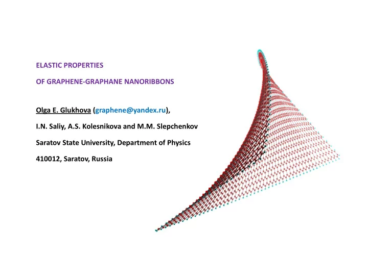
ELASTIC PROPERTIES OF GRAPHENE-GRAPHANE NANORIBBONS Olga E. Glukhova (graphene@yandex.ru), I.N. Saliy, A.S. Kolesnikova and M.M. Slepchenkov Saratov State University, Department of Physics 410012, Saratov, Russia

2 Graphene-nanoribbons We have studied some graphene- graphane nanoribbons with length- to- width ratio L/D from 2 to 3.22. So, nanostructures with ratio L/D less than 3 are classified as nanoparticles, nanoribbons with ratio more than 3 are classified as nanoribbons.

3 Deformations and elastic properties: empirical study To describe the Computational method interaction between the The entire system energy is described by the atom and its sum of the binding energy E , the torsional environment we b energy and the van der Waals energy E introduce three different tors regions in topological E : vdW network (see Figure 1).    As shown in Fig.1, there E E E E . (1) tot b tors vdW Fig. 1. Three different are near (first), far (third) regions in topological and intermediate network of an atomic (second) regions about In order to study the elastic properties and structure atom with number i. deformations of graphene-graphane Atoms from near region are covalently bonded with nanoribbons we applied the empirical method atom i, atoms from other regions are non-bonded based on the bond-order potential developed by with atom i. The far region has no borders. Brenner ( ).

4 Each pair of covalently bonded atoms interacts The torsional potential is given by the formula via a potential-energy:       Nat 1       tors         E V ( ) .   Nat   tors ijkl     1   2             E V ( r ) B V ( r ) . (2)   i 1 j i k i , j l i , j , k b  R ij ij A ij  2     i 1 j ( i ) (3) This is the binding energy. Here V R is the tors  The torsional potential V ( ) is given as a ijkl repulsive pair term, V A is the attractive pair term, function of a dihedral angle ω. The torsion angle r is the distance between the atom with number i ij  is defined in the usual way as the angle ijkl and atom j from near region. The function B ij is the between the plane defined by the vectors r ik and r ij many-body term. This term was introduced to and that defined by r ij and r jl . Here atoms j and k describe the specificity of the σ–π interaction. So, are given from intermediate (second) region and the value of the binding energy depends on the the atom l is given from far region. position and chemical identity of atoms.

5 Van der Waals energy E vdW Van der Waals interaction energy may be described by the defines the interaction between Lennard-Jones, Morse, Buckingham potentials and so on. We have non-bonded atoms: implemented and compared Lennard-Jones and Morse potentials as functions to define the van der Waals energy. We use Morse potential that is given by   Nat 1        . E V ( r )         vdW vdW ij 2 2               i 1 j ( i ) V ( r ) D 1 exp ( r r ) 1 E exp ' r , Morse ij e ij e r ij (4) (5) where D is the average bond energy, E is the repulsion nucleus e r energy,  , '  - parameters.

6 1) Optimization of atomic structure by entire system energy minimization (Eq.1) on atomic coordinates (the atomic structure obtained from previous Algorithm of the optimization); calculation of the Young’s pseudo - 2) tension or compression of the atomic network of nanoribbon and modulus reoptimization of atomic structure with atoms fixed on the nanoribbon ends; 3) for the elastic tension of nanoribbon on 1% the Young’s pseudo -modulus is calculated on formula: F L  Y p , (6)  D L where a deformation force is given by  2 E  F . (7)  L  is the strain energy, namely, the total energy at a given axial strain Here E minus the total energy.

7 Fig.2. Young’s pseudo -modulus of the nanoribbons

8 We have compared the elastic properties of the carbon nanotube and the nanoribbon with the same width. We have calculated the Young’s pseudo-modulus of the nanotube (5,5) with the perimeter about 2.1 nm and of the armchair-nanoribbon with the width 2.3 nm. Young’s pseudo -modulus of the armchair-nanoribbon is more than modulus of the nanotube on 27 %. Fig.3. Strain energy of nanoribbons undergoing axial tension

9 a) Armchair-nanoribbons b) zigzag-nanoribbons Fig.4. Strain energy of nanoribbons undergoing axial tension

10 a) Armchair-nanoribbons b) zigzag-nanoribbons Fig.5. Strain energy of nanoribbons undergoing axial compression

11 Deformations and elastic properties: quantum study The TB method was earlier implemented to The wave functions can be approximated by  n  | study a stability of carbon. The energy of a system of linear combination ion cores and valence electrons is written as   E E E . (8) n       tot bond rep | C | , (10)   n l l  l Here the term E is the bond structure energy bond where    l is an orthogonal basis set, l is the  that is calculated as the sum of energies of the quantum number index and  labels the ions. For single-particle occupied states. Those single-particle carbon compounds the matrix elements are energies are known by solving the Schrodinger calculated as equation           p p p | n | , (9) H         n p r 4 p 4 1 0    3      3      V ( r ) V exp p , n       1         r p p   2 2      is the where H is the one-electron Hamiltonian, n (11) energy of the n th single-particle state. where r is the distance between atoms.

12 0 Term E in Eq.(8) is the phenomenon energy rep The values of the parameters V  , the atomic that is a repulsive potential. It can be expressed as a terms and p n for carbon compounds are given in sum of two-body potentials as table.     E V r , (12)  rep rep Table 1     , 0  , 0  , V V  , эВ  , эВ sp pp 0  , эВ V  , эВ 0 is pair potential between atoms at  V p s where V pp ss rep эВ эВ and  . This two-body potential describes an -10,932 -5,991 -4,344 3,969 5,457 -1,938 interaction between bonded and nonbonded atoms and is presented in [8] p 1 p 2 , Å p 3 , Å p 4 p 5 , эВ p 6 2,796 2,32 1,54 22 10,92 4,455     p p p         p p r 4 4 6   3 3            V ( r ) p exp p     Parameters were fitted from experimental data for rep 5 6     r  p   p    2 2   fullerenes and carbon nanotubes. Transferability to other   carbon compounds was tested by comparison with ab (13) initio calculations and experiments. where i and j are orbital moments of wave Our transferable tight-binding potential can correctly function,  presents the bond type (  or  ). reproduce changes in the electronic configuration as a function of the local bonding geometry around each carbon atom.

13 All s- and P-orbitals are given in the real Cartesian co- ordinates system. To correctly reproduce changes in the electronic configuration of the local bonding geometry around each atom we have defined P-orbital as the axial vector. Each axial vector makes the angle with an direction R ij (α, β, θ ) and may be written as the geometrical sum of the two vectors:           P P P P P P  ,  , (14) x xD x y yD y      P P P  . z zD z    P P P Here , , are projections to an iteratomic xD yD zD  P direction,  … are projections to an orthogonal x direction. Fig. 6. Schematic representation of the interaction So, to describe the interaction between P z and P x (see of P z - and P x - orbital. Fig.) we must write:            P P P P P P   x z xD zD x z . (15)   - bonding - bonding