Efficient Search for Inputs Causing High Floating-point Errors - PowerPoint PPT Presentation
Efficient Search for Inputs Causing High Floating-point Errors Wei-Fan Chiang , Ganesh Gopalakrishnan, Zvonimir Rakamari , and Alexey Solovyev School of Computing, University of Utah, Salt Lake City, UT Supported in part by NSF grants ACI
Efficient Search for Inputs Causing High Floating-point Errors Wei-Fan Chiang , Ganesh Gopalakrishnan, Zvonimir Rakamarić , and Alexey Solovyev School of Computing, University of Utah, Salt Lake City, UT Supported in part by NSF grants ACI 1148127, CCF 1255776, CCF 1302449 and CCF 1346756.
Floating-point Computations in Sequential and Parallel Software • Important applications such as weather prediction are accuracy-critical • Everyday applications (e.g. cell-phone apps) run at lower FP precision • Challenge : Knowing whether they give imprecise results for any input 1 Photo courtesy to drroyspencer.com, aptito.com/blog, and itunes.apple.com.
Dangers of Inadequate or Inconsistent Precision • Patriot Missile Failure in 1991. – Miscalculated distance due to floating-point error. • Inconsistent FP Calculations [Meng et al, XSEDE ‘13] P = 0.421874999999999944488848768742172978818416595458984375 C = 0.0026041666666666665221063770019327421323396265506744384765625 Compute: floor( P / C ) Xeon Xeon Expecting Sent Phi 161 msgs 162 msgs P / C = 161.9999… P / C = 162 floor( P / C ) = 161 floor( P / C ) = 162 2
Problem Addressed • How to tell which inputs maximize error? • This is important for many reasons: – Characterize libraries precisely – Support tuning precision – Help decide where error-compensation is productive Relative Error Feasible Inputs 3
Difficulties • Large code-sizes • Presence of non-linear operators • Presence of data-dependent conditionals • Concurrency (schedules may affect results) Relative Error Feasible Inputs 4
Main Contribution • A practical technique for reliable precision estimation for sequential and parallel programs. – Search based input generation. – Handles diverse operations. – Improves scalability. • Usage scenarios: – Precision bottleneck detection. – Auto-tuning. 5
Previous Work • Over-approximation based (false alarms likely) : – Interval arithmetic: Examples • x in [-1, 2] and y in [2, 5]. Then (x * y) returned as [-5, 10]. • x in [-1, 1]. Then (x – x) returned as [-2, 2] (must be 0) – Affine arithmetic: Basic idea • Each number is represented by a polynomial. • Linear approximation of non-linear operation. – SMT • Encodes error bound described in IEEE-754 standard. • Under-approximation based (no false alarms): – Random testing. 6
Illustration of Interval Arithmetic 1. float x0 , x1, x2 in [1.0, 2.0] 2. float p0 = (x0 + x1) – x2 3. float p1 = (x1 + x2) – x0 4. float p2 = (x2 + x0) – x1 5. float sum = (p0 + p1) + p2 6. Error? sum // (x0 + x1) + x2 Exact Interval Arithmetic Affine Arithmetic SMT based (Gappa) (SmartFloat) Value of [3.0, 6.0] [0.0, 9.0] [3.0, 6.0] [3.0, 6.0] sum Error on ? Infinite 1.0362e-15 4.9960e-15 sum 7
Illustration of Affine Arithmetic / SMT 1. float xi in [1.0, 3.0] // 0 ≤ i ≤ 7 2. float sum = summation of xi 3. Consider xi in [1.0, 2.0] 4. Error? sum Exact Interval Arithmetic Affine Arithmetic SMT based (Gappa) (SmartFloat) Value of [8.0, 16.0] [8.0, 16.0] N/A [8.0, 16.0] sum Error on ? 7.7548e-16 N/A Timeout sum 8
Previous Work • Over-approximation: Interval Affine SMT based Arithmetic Arithmetic Poor scalability √ Overly pessimistic results √ Limited support for √ √ √ non-linear operation Limited support for √ conditionals • Our overall approach: Under-approximation based – Naïve Random Testing produces VERY LOOSE lower bounds – Our focus : How to produce tight lower-bounds ? 9
Why do we base our approach on Guided Random Testing? • Seems to be the only approach that can handle – Large Programs – Non-linear operators – Data dependent conditionals No “closed form” solutions are possible • At present, designers have no tools that can analyze programs with these features – Ours is the first practical tool in this area 10
Precision Measurement by Random Testing Low Precision Low Precision Result Program configuration X0 Error Calculation* X1 X2 High Precision High Precision Program Result * “Error” = Relative Error (See paper for details) 11
Search Based Random Testing • Our Contribution : Random Testing with Good Guidance Heuristics can Outperform Naïve Random • We propose Binary Guided Random Testing Pure Search Based Real Max. Over-approximation Random Random Error 0 ∞ ? 12
Search Based Random Testing • Randomly sample inputs around “ sour-spots! ” – A “sour - spot” causes highly imprecise program output. – Definition of “Configuration:” An assignment from input variables to their probing intervals. Configuration: 0.0 1.0 X0 Program Result 1.1 2.2 X1 2.3 3.3 X2 13
Search Based Random Testing • Randomly sample inputs around “ sour-spots! ” – A “sour - spot” causes highly imprecise program output. – Definition of “Configuration:” An assignment from input variables to their probing intervals. Configuration: X0 = 0.5 0.0 0.5 1.0 X1 = 1.5 X0 X2 = 3.0 Imprecise Program 1.1 1.5 2.2 Result X1 2.3 3.0 3.3 X2 14
Search Based Random Testing • Randomly sample inputs around “ sour-spots! ” – A “sour - spot” causes highly imprecise program output. – Definition of “Configuration:” An assignment from input variables to their probing intervals. New Configuration: 0.4 0.6 Result for X0 New Program 1.4 1.6 X1 Config. 2.9 3.1 X2 15
Importance of Selecting Good Configurations Good Conf. x0 x1 Original Conf. x0 x1 Bad Conf. x0 x1 Number of Samples 16
Binary Guided Random Testing: Search and Test Around Sour-spots • Key Observations: – “Sour spots” can be improved with more probing – Configurations can be ranked without too much probing • The optimization problem: – Find a configuration that contains inputs causing high floating-point errors. – We propose Binary Guided Random Testing (BGRT). – We compared BGRT against other search methods, obtaining encouraging results 17
High-level View of BGRT Original Conf. Init Derive Configuration to Generate Candidates sub- sub- ..... conf. 1 conf. n Candidates Program 18
High-level View of BGRT Original Conf. Init Derive Configuration to Generate Candidates Choose the BEST Sub-conf. sub- sub- ..... conf. 1 conf. n Evaluate Candidates Program 19
High-level View of BGRT Original Conf. Init Derive Configuration to Generate Candidates Choose the BEST Sub-conf. sub- sub- ..... conf. 1 conf. n Evaluate Candidates Program For each sub-conf., sample few inputs. Also Record the detected highest error. 20
High-level View of BGRT Original Conf. Init sub-conf. k The BEST among Derive Configuration to candidates Generate Candidates Choose the BEST Sub-conf. sub- sub- ..... conf. 1 conf. n Evaluate Candidates Program For each sub-conf., sample few inputs. Also Record the detected highest error. 21
High-level View of BGRT Original Restart? Conf. Init sub-conf. k The BEST among Derive Configuration to candidates Generate Candidates Choose the BEST Sub-conf. sub- sub- ..... conf. 1 conf. n Evaluate Candidates Program For each sub-conf., sample few inputs. Also Record the detected highest error. 22
High-level View of BGRT Original Restart? Conf. Init OR sub-conf. k The BEST among Derive Configuration to candidates Generate Candidates Choose the BEST Sub-conf. sub- sub- ..... conf. 1 conf. n Evaluate Candidates Program For each sub-conf., sample few inputs. Also Record the detected highest error. 23
A Closer View of BGRT X0 X1 X2 X0 X1 X2 • Partition the variables (with their ranges). 24
A Closer View of BGRT X0 X1 X2 X0 X1 X2 X0 X0 X1 X1 X2 X2 • Shrink variables’ ranges. – Each partition generates its “ upper ” and “ lower ” sub - partitions. 25
A Closer View of BGRT X0 X1 X2 X0 X1 X2 X0 X0 X1 X1 X2 X2 X0 X0 X0 X0 X1 X1 X1 X1 X2 X2 X2 X2 26
A Closer View of BGRT X0 X1 X2 Candidates These candidates are evaluated using random sampled inputs. X0 X0 X0 X0 X1 X1 X1 X1 X2 X2 X2 X2 27
Other Search Strategies We Investigated • Iterated Local Search (ILS) • Particle Swarm Optimization (PSO) • Our results suggest BGRT as the better search strategy for precision measurement. – Focuses the search near sour-spots. • Website for additional documents: – www.cs.utah.edu/fv/Gauss/Pages/grt 28
Experimental Results • Comparison among search strategies – Unguided Random Testing (URT), BGRT, ILS, and PSO • Benchmarks – Various reduction-tree shapes – Direct Quadrature Method of Moments (DQMOM) – GPU primitives 29
Evaluation of BGRT (Reductions) • Imbalanced reduction (IBR) • Balanced reduction (BR) • Compensated imbalanced reduction (IBRK) • Over-approximation techniques cannot report that the compensated reduction is the most precise. Balanced Reduction Imbalanced Reduction ((v0 + v1) + (v2 + v3)) (((v0 + v1) + v2) + v3) ((v0 + v1) + v2) v3 (v0 + v1) (v2 + v3) (v0 + v1) v2 v0 v1 v2 v3 v0 v1 30
Recommend
More recommend
Explore More Topics
Stay informed with curated content and fresh updates.
