EECS E6870 - Speech Recognition Administrivia Lecture 2 Feature - PowerPoint PPT Presentation
Outline of Todays Lecture EECS E6870 - Speech Recognition Administrivia Lecture 2 Feature Extraction Brief Break Dynamic Time Warping Stanley F . Chen, Michael A. Picheny
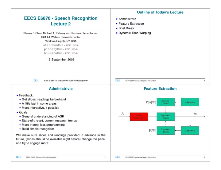
� ✟ ✆ ✂ ✁ ✝✞ ✄☎ ☛ ✠✡ Outline of Today’s Lecture EECS E6870 - Speech Recognition ■ Administrivia Lecture 2 ■ Feature Extraction ■ Brief Break ■ Dynamic Time Warping Stanley F . Chen, Michael A. Picheny and Bhuvana Ramabhadran IBM T.J. Watson Research Center Yorktown Heights, NY, USA stanchen@us.ibm.com picheny@us.ibm.com bhuvana@us.ibm.com 15 September 2009 EECS E6870: Advanced Speech Recognition EECS E6870: Advanced Speech Recognition 1 Administrivia Feature Extraction ■ Feedback: ● Get slides, readings beforehand ● A little fast in some areas ● More interactive, if possible ■ Goals: ● General understanding of ASR ● State-of-the-art, current research trends ● More theory, less programming ● Build simple recognizer Will make sure slides and readings provided in advance in the future, (slides should be available night before) change the pace, and try to engage more. EECS E6870: Advanced Speech Recognition 2 EECS E6870: Advanced Speech Recognition 3
✟ ✝✞ ✆ ☛ ✠✡ � ✁ ✂ ✄☎ What will be “Featured”? Goals of Feature Extraction ■ Linear Prediction (LPC) ■ What do YOU think the goals of Feature Extraction should be? ■ Mel-Scale Cepstral Coefficients (MFCCs) ■ Perceptual Linear Prediction (PLP) ■ Deltas and Double-Deltas ■ Recent developments: Tandem models Figures from Holmes, HAH or R+J unless indicated otherwise. EECS E6870: Advanced Speech Recognition 4 EECS E6870: Advanced Speech Recognition 5 What are some possibilities? Goals of Feature Extraction ■ Capture essential information for sound and word identification ■ What sorts of features would you extract? ■ Compress information into a manageable form ■ Make it easy to factor out irrelevant information to recognition such as long-term channel transmission characteristics. EECS E6870: Advanced Speech Recognition 6 EECS E6870: Advanced Speech Recognition 7
✟ � ✁ ✂ ☛ ✝✞ ✆ ✠✡ ✄☎ What are some possibilities? Historical Digression ■ Model speech signal with a parsimonious set of parameters that ■ 1950s-1960s - Analog Filter Banks best represent the signal. ■ 1970s - LPC ■ Use some type of function approximation such as Taylor or ■ 1980s - LPC Cepstra Fourier series ■ 1990s - MFCC and PLP ■ Exploit correlations in the signal to reduce the the number of ■ 2000s - Posteriors, and multistream combinations parameters Sounded good but never made it ■ Exploit knowledge of perceptual processing to eliminate irrelevant variation - for example, fine frequency structure at ■ Articulatory features high frequencies. ■ Neural Firing Rate Models ■ Formant Frequencies ■ Pitch (except for tonal languages such as Mandarin) EECS E6870: Advanced Speech Recognition 8 EECS E6870: Advanced Speech Recognition 9 Three Main Schemes Pre-Emphasis Purpose: Compensate for 6dB/octave falloff due to glottal-source and lip-radiation combination. Assume our input signal is x [ n ] . Pre-emphasis is implemented via very simple filter: y [ n ] = x [ n ] + ax [ n − 1] To analyze this, let’s use the “Z-Transform” introduced in Lecture 1. Since x [ n − 1] = z − 1 x [ n ] we can write Y ( z ) = X ( z ) H ( z ) = X ( z )(1 + az − 1 ) If we substitute z = e jω , we can write | H ( e jω ) | 2 | 1 + a (cos ω − j sin ω ) | 2 = 1 + a 2 + 2 a cos ω = EECS E6870: Advanced Speech Recognition 10 EECS E6870: Advanced Speech Recognition 11
✟ ✂ ✆ ☛ ✠✡ ✄☎ ✝✞ � ✁ or in dB Uses are: ■ Improve LPC estimates (works better with “flatter” spectra) 10 log 10 | H ( e jω ) | 2 = 10 log 10 (1 + a 2 + 2 a cos ω ) ■ Reduce or eliminate DC offsets ■ Mimic equal-loudness contours (higher frequency sounds appear “louder” than low frequency sounds for the same amplitude) For a > 0 we have a low-pass filter and for a < 0 we have a high-pass filter, also called a “pre-emphasis” filter because the frequency response rises smoothly from low to high frequencies. EECS E6870: Advanced Speech Recognition 12 EECS E6870: Advanced Speech Recognition 13 Basic Speech Processing Unit - the Frame Block input into frames consisting of about 20 msec segments (200 samples at a 10 KHz sampling rate). More specifically, define x m [ n ] = x [ n − mF ] w [ n ] How do we choose the window w [ n ] , the frame spacing, F , and the window length, N ? as frame m to be processed where F is the spacing frames and ■ Experiments in speech coding intelligibility suggest that F w [ n ] is our window of length N . should be around 10 msec. For F greater than 20 msec one starts hearing noticeable distortion. Less and things do not appreciably improve. Let us also assume that x [ n ] = 0 for n < 0 and n > L − 1 . For ■ From last week, we know that Hamming windows are good. consistency with all the processing schemes, let us assume x has So what window length should we use? already been pre-emphasized. EECS E6870: Advanced Speech Recognition 14 EECS E6870: Advanced Speech Recognition 15
� ✝✞ ✂ ☛ ✠✡ ✄☎ ✆ ✁ ✟ ■ If too long, vocal tract will be non-stationary; smooth out Effects of Windowing transients like stops. ■ If too short, spectral output will be too variable with respect to window placement. Usually choose 20-25 msec window length as a compromise. EECS E6870: Advanced Speech Recognition 16 EECS E6870: Advanced Speech Recognition 17 ■ What do you notice about all these spectra? EECS E6870: Advanced Speech Recognition 18 EECS E6870: Advanced Speech Recognition 19
✟ ✆ ☛ ✠✡ � ✁ ✂ ✄☎ ✝✞ Optimal Frame Rate Linear Prediction ■ Few studies of frame rate vs. error rate ■ Above curves suggest that the frame rate should be one-third of the frame size EECS E6870: Advanced Speech Recognition 20 EECS E6870: Advanced Speech Recognition 21 Linear Prediction - Motivation Linear Prediction The linear prediction model assumes that x [ n ] is a linear combination of the p previous samples and an excitation e [ n ] The above model of the vocal tract matches observed data quite p � x [ n ] = a [ j ] x [ n − j ] + Ge [ n ] well, at least for speech signals recorded in clean environments. It j =1 can be shown that associated the above vocal tract model can be associated with a filter H ( z ) with a particularly simple time-domain e [ n ] is either a string of (unit) impulses spaced at the fundamental interpretation. frequency (pitch) for voiced sounds such as vowels or (unit) white EECS E6870: Advanced Speech Recognition 22 EECS E6870: Advanced Speech Recognition 23
✟ � ✝✞ ✆ ✁ ✂ ✄☎ ✠✡ ☛ noise for unvoiced sounds such as fricatives. Solving the Linear Prediction Equations Taking the Z-transform, It seems reasonable to find the set of a [ j ] s that minimize the prediction error G X ( z ) = E ( z ) H ( z ) = E ( z ) 1 − � p p j =1 a [ j ] z − j ∞ � � a [ j ] x [ n − j ]) 2 ( x [ n ] − n = −∞ j =1 where H ( z ) can be associated with the (time-varying) filter associated with the vocal tract and an overall gain G . If we take derivatives with respect to each a [ i ] in the above equation and set the results equal to zero we get a set of p equations indexed by i : p � a [ j ] R ( i, j ) = R ( i, 0) , 1 ≤ i ≤ p j =1 where R ( i, j ) = � n x [ n − i ] x [ n − j ] . In practice, we would not use the potentially infinite signal x [ n ] but EECS E6870: Advanced Speech Recognition 24 EECS E6870: Advanced Speech Recognition 25 the individual windowed frames x m [ n ] . Since x m [ n ] is zero outside The Levinson-Durbin Recursion the window, R ( i, j ) = R ( j, i ) = R ( | i − j | ) where R ( i ) is just the The previous set of linear equations (actually, the matrix autocorrelation sequence corresponding to x m ( n ) . This allows us associated with the equations) is called Toeplitz and can easily to write the previous equation as be solved using the “Levinson-Durbin recursion” as follows: p Initialization E 0 = R (0) � a [ j ] R ( | i − j | ) = R ( i ) , 1 ≤ i ≤ p Iteration. For i = 1 , . . . , p do j =1 i − 1 a much simpler and regular form. � a i − 1 [ j ] R ( | i − j | )) /E i − 1 k [ i ] = ( R ( i ) − j =1 a i [ i ] = k [ i ] a i [ j ] a i − 1 [ j ] − k [ i ] a i − 1 [ i − j ] , 1 ≤ j < i = E i (1 − k [ i ] 2 ) E i − 1 = End. a [ j ] = a p [ j ] and G 2 = E p . Note this is an O ( n 2 ) algorithm rather than O ( n 3 ) and made possible by the Toeplitz structure of EECS E6870: Advanced Speech Recognition 26 EECS E6870: Advanced Speech Recognition 27
Recommend
More recommend
Explore More Topics
Stay informed with curated content and fresh updates.
