EconS 424: Strategy and Game Theory Oligopoly games with incomplete - PDF document

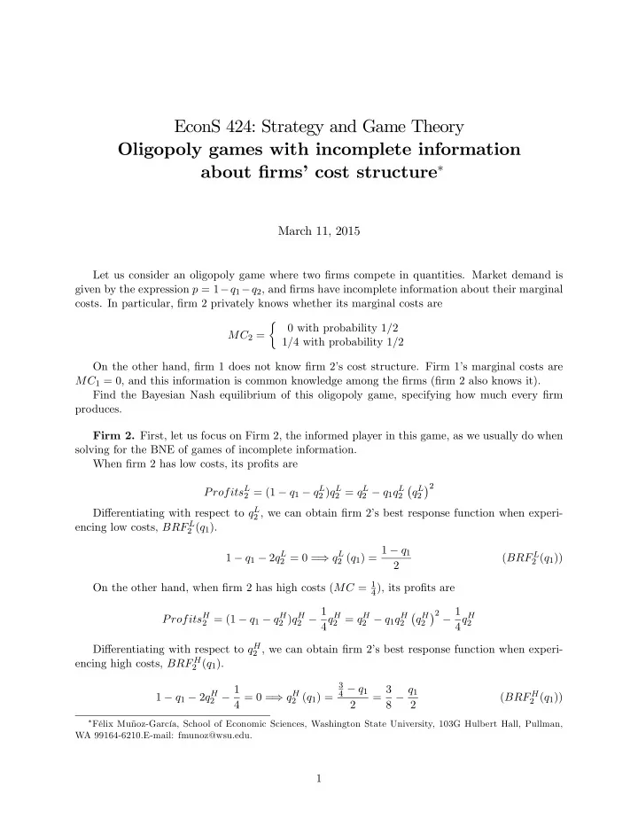
EconS 424: Strategy and Game Theory Oligopoly games with incomplete information about …rms’ cost structure � March 11, 2015 Let us consider an oligopoly game where two …rms compete in quantities. Market demand is given by the expression p = 1 � q 1 � q 2 , and …rms have incomplete information about their marginal costs. In particular, …rm 2 privately knows whether its marginal costs are � 0 with probability 1/2 MC 2 = 1 = 4 with probability 1/2 On the other hand, …rm 1 does not know …rm 2’s cost structure. Firm 1’s marginal costs are MC 1 = 0 , and this information is common knowledge among the …rms (…rm 2 also knows it). Find the Bayesian Nash equilibrium of this oligopoly game, specifying how much every …rm produces. Firm 2. First, let us focus on Firm 2, the informed player in this game, as we usually do when solving for the BNE of games of incomplete information. When …rm 2 has low costs, its pro…ts are � � 2 Profits L 2 = (1 � q 1 � q L 2 ) q L 2 = q L 2 � q 1 q L q L 2 2 Di¤erentiating with respect to q L 2 , we can obtain …rm 2’s best response function when experi- encing low costs, BRF L 2 ( q 1 ) . 2 ( q 1 ) = 1 � q 1 1 � q 1 � 2 q L ) q L ( BRF L 2 = 0 = 2 ( q 1 ) ) 2 On the other hand, when …rm 2 has high costs ( MC = 1 4 ), its pro…ts are � � 2 � 1 2 � 1 Profits H 2 = (1 � q 1 � q H 2 ) q H 4 q H 2 = q H 2 � q 1 q H q H 4 q H 2 2 2 Di¤erentiating with respect to q H 2 , we can obtain …rm 2’s best response function when experi- encing high costs, BRF H 2 ( q 1 ) . 3 2 � 1 4 � q 1 = 3 8 � q 1 1 � q 1 � 2 q H ) q H ( BRF H 4 = 0 = 2 ( q 1 ) = 2 ( q 1 ) ) 2 2 � Félix Muñoz-García, School of Economic Sciences, Washington State University, 103G Hulbert Hall, Pullman, WA 99164-6210.E-mail: fmunoz@wsu.edu. 1

Firm 1. Let us now analyze Firm 1 (the uninformed player in this game). First note that its pro…ts must be expressed in expected terms, since …rm 1 does not know whether …rm 2 has low or high costs. Profits 1 = 1 + 1 2(1 � q 1 � q L 2(1 � q 1 � q H 2 ) q 1 2 ) q 1 | {z } | {z } if low costs if high costs Rearranging, � 1 � � � 2 � q L 2 � q H 1 � q 1 � q L 2 � q H 2 � q 1 2 + 1 2 � q 1 2 2 2 2 Profits 1 = q 1 = q 1 2 2 = q 1 � ( q 1 ) 2 � q L 2 q 1 � q H 2 2 2 q 1 Di¤erentiating with respect to q 1 , we can obtain …rm 1’s best response function, BRF 1 ( q L 2 ; q H 2 ) : Note that we do not have to di¤erentiate for the case of low and high costs, since …rm 1 does not observe such information). In particular, 1 � 2 q 1 � q L 2 � q H � � 2 � q L 2 � q H = 1 2 2 q L 2 ; q H 2 2 ( BRF 1 ( q L 2 ; q H 2 = 0 = ) q 1 2 ) ) 2 2 � After …nding the best response functions for both types of Firm 2 and for the unique type of Firm 1 we are ready to plug the …rst two BRFs into the latter. Speci…cally, 1 � q 1 8 � q 1 3 q 1 = 1 2 2 2 � � 2 2 which simpli…es to q 1 = 1 16 + 8 16 q 1 And solving for q 1 , we …nd q 1 = 1 8 . � With this information, it is easy to …nd the particular level of production for …rm 2 when experiencing low marginal costs, = 1 � 1 2 ( q 1 ) = 1 � q 1 = 7 q L 8 2 2 16 � As well as the level of production for …rm 2 when experiencing high marginal costs, 1 2 ( q 1 ) = 3 2 = 5 q H 8 8 � 16 � Therefore, the Bayesian Nash equilibrium of this oligopoly game with incomplete information about …rm 2’s marginal costs prescribes the following production levels � 3 � � � 8 ; 7 16 ; 5 q 1 ; q L 2 ; q H = 2 16 2

EconS 424: Strategy and Game Theory Oligopoly games with incomplete information d � about mar k et d eman March 11, 2015 Let us consider an oligopoly game where two …rms compete in quantities. Both …rms have the same marginal costs, MC = $ � , but they are asymmetrically informed about the actual state of market demand. In particular, Firm 2 does not know what is the actual state of demand, but knows that it is distributed with the following probability distribution � 10 � Q with probability 1/2 p ( Q ) = 5 � Q with probability 1/2 On the other hand, …rm 1 knows the actual state of market demand, and …rm 2 knows that …rm 1 knows this information (i.e., it is common knowledge among the players). Firm 1. First, let us focus on Firm 1, the informed player in this game, as we usually do when solving for the BNE of games of incomplete information. When …rm 1 observes a high demand market its pro…ts are Q ) q H 1 � 1 q H Profits 1 = (10 � 1 (10 � q H 1 � q 2 ) q H 1 � q H = 1 � � 2 � q 2 q H 10 q H q H 1 � 1 q H = 1 � 1 1 Di¤erentiating with respect to q H 1 , we can obtain …rm 1’s best response function when experi- encing low costs, BRF H 1 ( q 2 ) . 1 ( q 2 ) = 4 : 5 � q 2 10 � 2 q H ) q H ( BRF H 1 � q 2 � 1 = 0 = 1 ( q 2 ) ) 2 On the other hand, when …rm 1 observes a low demand market its pro…ts are � � 2 � q 2 q L Profits 1 = (5 � q L 1 � q 2 ) q L 1 � 1 q L 1 = 5 q L q L 1 � 1 q L 1 � 1 1 Di¤erentiating with respect to q L 1 , we can obtain …rm 1’s best response function when experi- encing high costs, BRF L 1 ( q 2 ) . 1 ( q 2 ) = 2 � q 2 5 � 2 q L ) q L ( BRF L 1 � q 2 � 1 = 0 = 1 ( q 2 ) ) 2 � Félix Muñoz-García, School of Economic Sciences, Washington State University, 103G Hulbert Hall, Pullman, WA 99164-6210.E-mail: fmunoz@wsu.edu. 1

Firm 2. Let us now analyze Firm 2 (the uninformed player in this game). First note that its pro…ts must be expressed in expected terms, since …rm 2 does not know whether market demand is high or low. � � Profits 2 = 1 + 1 (10 � q H (5 � q L � � 1 � q 2 ) q 2 � 1 q 2 1 � q 2 ) q 2 � 1 q 2 2 | {z } 2 | {z } demand is high demand is low Rearranging, Profits 2 = 1 + 1 1 q 2 � ( q 2 ) 2 � q 2 1 q 2 � ( q 2 ) 2 � q 2 h i h i 10 q 2 � q H 5 q 2 � q L 2 2 Di¤erentiating with respect to q 2 , we can obtain …rm 2’s best response function, BRF 2 ( q L 1 ; q H 1 ) : Note that we do not have to di¤erentiate for the case of low and high demand, since …rm 2 does not observe such information). In particular, � � 1 + 1 10 � q H 5 � q L � � 1 � 2 q 2 � 1 1 � 2 q 2 � 1 = 0 2 2 Rearraging, 13 � q H 1 � 4 q 2 � q L 1 = 0 And solving for q 2 , � � = 13 � q L 1 � q H � � � � q L 1 ; q H 1 q L 1 + q H q L 1 ; q H q 2 = 3 : 25 � 0 : 25 ( BRF 2 ) 1 1 1 4 � After …nding the best response functions for both types of Firm 1 and for the unique type of Firm 2 we are ready to plug the …rst two BRFs into the latter. Speci…cally, 0 1 2 � q 2 4 : 5 � q 2 B h i h i C q 2 = 3 : 25 � 0 : 25 + B C 2 2 B C | {z } | {z } @ A q L q H 1 1 which simpli…es to q 2 = 3 : 25 � 1 : 625 + 0 : 25 q 2 And solving for q 2 , we …nd q 2 = 2 : 167 . � With this information, it is easy to …nd the particular level of production for …rm 1 when experiencing low market demand, 1 ( q 2 ) = 2 � q 2 2 = 2 � 2 : 167 q L = 0 : 2 9 � � � As well as the level of production for …rm 1 when experiencing high market demand, 1 ( q 2 ) = 4 : 5 � q 2 2 = 4 : 5 � 2 : 167 q H = 3 : 4167 2 � Therefore, the Bayesian Nash equilibrium (BNE) of this oligopoly game with incomplete information about market demand prescribes the following production levels � � q H 1 ; q L 1 ; q 2 = (3 : 416 ; 0 : � ; 2 : 167) 9 � 2