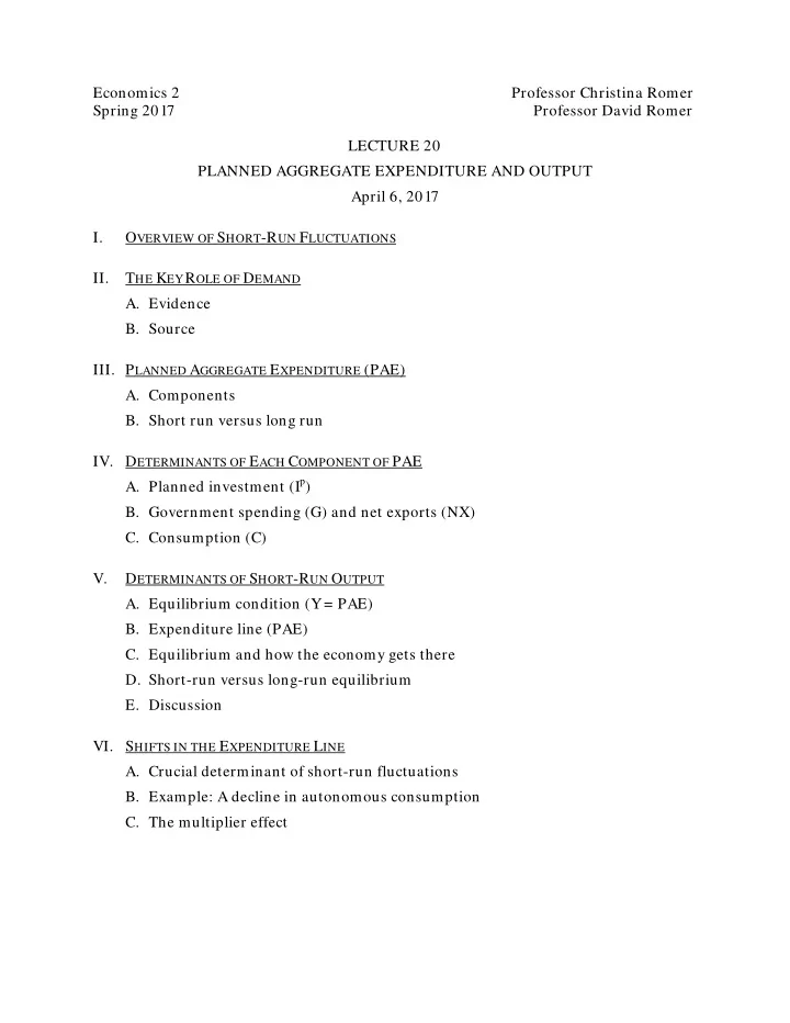

Economics 2 Professor Christina Romer Spring 2017 Professor David Romer LECTURE 20 PLANNED AGGREGATE EXPENDITURE AND OUTPUT April 6, 2017 I. O VERVIEW OF S HORT -R UN F LUCTUATIONS II. T HE K EY R OLE OF D EMAND A. Evidence B. Source III. P LANNED A GGREGATE E XPENDITURE (PAE) A. Components B. Short run versus long run IV. D ETERMINANTS OF E ACH C OMPONENT OF PAE A. Planned investment (I p ) B. Government spending (G) and net exports (NX) C. Consumption (C) V. D ETERMINANTS OF S HORT -R UN O UTPUT A. Equilibrium condition (Y = PAE) B. Expenditure line (PAE) C. Equilibrium and how the economy gets there D. Short-run versus long-run equilibrium E. Discussion VI. S HIFTS IN THE E XPENDITURE L INE A. Crucial determinant of short-run fluctuations B. Example: A decline in autonomous consumption C. The multiplier effect
Economics 2 Christina Romer Spring 2017 David Romer L ECTURE 20 Planned Aggregate Expenditure and Output April 6, 2017
Announcements • We have handed out Problem Set 5. • It is due at the start of lecture on Thursday, April 13 th . • Problem set work session next Tuesday, April 11 th , 5:00–7:00 p.m. in 648 Evans. Research paper reading for next time. • • Romer and Romer, “The Macroeconomic Effects of Tax Changes.”
I. O VERVIEW OF S HORT -R UN F LUCTUATIONS
Real GDP in the United States, 1950–2016 Source: FRED (Federal Reserve Economic Data); data from Bureau of Economic Analysis.
Short-Run Fluctuations • Times when output moves above or below potential (booms and recessions). • Recessions are costly and very painful to the people affected.
The U.S. Unemployment Rate, 1948–2017 Source: FRED; data from Bureau of Labor Statistics.
II. T HE K EY R OLE OF D EMAND
Key Determinant of Output in the Short Run • In the short run, aggregate output is determined by demand. • Three terms that mean the same thing: • Planned aggregate expenditure • Planned spending • Planned aggregate demand • All three terms refer to the total amount that people in the economy plan to buy (or spend).
Evidence on the Key Role of Demand • Historical experience • Academic research
Why is output determined by demand in the short run? • Nominal rigidities (inflation doesn’t change substantially in the short run). • Due to limited information, menu costs, long-term contracts, or other factors.
III. P LANNED A GGREGATE E XPENDITURE
Components of Planned Aggregate Expenditure (PAE) • Consumption (C) • Planned investment (I p ) • Government purchases (G) • Net exports (NX) PAE = C + I p + G + NX
Short Run versus Long Run • In the short run: • PAE can be anything. • Output responds to match PAE. • In the long run: • Output is at Y* (determined by normal technology, capital, and employment). • PAE adjusts to equal Y*. • Movement in r brings this about.
IV. D ETERMINANTS OF E ACH C OMPONENT OF PAE
Determinants of Planned Investment (I p ) • Real interest rate (r) • Expectations (“animal spirits”) • We talk about “planned investment” because we are leaving out the unplanned investment in inventories that happens when PAE is different from actual output.
Determinants of Government Purchases (G) • Politics • Wars, natural disasters We take G as given.
Determinants of Net Exports (NX) • For now we are assuming they are just given. • Will discuss the economic determinants later in the course.
Determinants of Consumption (C) • Real interest rate (r) • Expectations (“consumer confidence”) • Wealth • Disposable income
Consumption and Disposable Income • Aggregate income: Same as aggregate output (Y) • Aggregate tax payments: Same as government tax revenues (T) • Aggregate disposable income: Y−T • Consumption function: C = f(Y−T) • Sometimes written in the particular form: � + c·(Y−T) C = C � is positive and c is between 0 and 1) (where C
Consumption Function C = C + c ·(Y−T) C C slope = c C Y−T
Consumption Function C = C + c·( Y−T) • Autonomous consumption: The part of consumption that does not vary with income (C). • Marginal propensity to consume (MPC): The change in planned consumption due to a change in disposable income (c).
Consumption and Disposable Income Source: Frank, Bernanke, Antonovics, and Heffetz, “Principles of Economics.”
V. D ETERMINATION OF S HORT -R UN O UTPUT
45-degree Line • Captures the equilibrium condition that Y=PAE. • Also reflects the empirical/behavioral reality that output responds to planned spending in the short run.
45-degree Line PAE Y=PAE 45° Y
Expenditure Line • Captures the fact that planned aggregate spending is a function of total income (which is the same as total output). • PAE = C + I p + G + NX, where C = f(Y−T).
Expenditure Line PAE PAE = C + I p + G + NX C Y The slope of the expenditure line (PAE) is the MPC.
Determination of Short-Run Output • Output in the short run is determined by the intersection of the 45-degree line and the expenditure line.
Determination of Short-Run Output PAE Y=PAE PAE Y 1 Y Sometimes called the “Keynesian Cross” diagram.
How does the economy get to short-run equilibrium? PAE Y=PAE PAE At Y 3 , unintended negative inventory At Y 2 , unintended inventory investment leads firms to increase investment leads firms to cut production. production. Y 3 Y 1 Y 2 Y
Long-Run Equilibrium PAE Y=PAE PAE Y* Y In the long run, PAE=Y and PAE cross at Y* (potential output).
VI. S HIFTS IN THE E XPENDITURE L INE
Crucial Determinant of Short-Run Fluctuations: Shifts in the Expenditure Line • Expenditure line (PAE) shows how planned spending varies with output. • Anything that changes planned spending other than output, will shift the curve. • If the expenditure line shifts, short-run equilibrium output will change.
Example: A Fall in Autonomous Consumption • A fall in consumption not caused by a fall in output. • A decline in the intercept of the consumption function (C).
Source: Federal Reserve Bank of St. Louis, FRED. Great Crash of the Stock Market in October 1929 Dow Jones Industrial Average (Index) 100 150 200 250 300 350 400 50 0 Dec-14 Dec-15 Dec-16 Dec-17 Dec-18 Dec-19 Dec-20 Dec-21 Dec-22 Dec-23 September 1929 Dec-24 Dec-25 Dec-26 Dec-27 Dec-28 Dec-29 Dec-30 Dec-31 Dec-32 Dec-33 Dec-34 Dec-35
Why might a fall in stock prices reduce consumer spending (at a given level of output)? • Reduction in wealth makes consumers feel poorer. • Fall in stock prices makes consumers pessimistic (lowers consumer confidence). • Stock price volatility causes uncertainty and leads to “wait and see” behavior.
The Collapse of Consumer Spending in Late 1929 Source: Christina Romer, “The Great Crash and the Onset of the Great Depression.”
A Fall in Autonomous Consumption C C 1 C 2 C 1 C 2 Y−T
A Fall in Autonomous Consumption PAE Y=PAE PAE 1 PAE 2 Y 2 Y* Y
Real GDP, 1909–1939 1300 1200 Real GDP in Chained 2009 Dollars 1929 1100 1000 900 800 700 600 500 400 1909 1911 1913 1915 1917 1919 1921 1923 1925 1927 1929 1931 1933 1935 1937 1939 Source: Christina Romer, “The Prewar Business Cycle Reconsidered,” and BEA.
The Multiplier Effect PAE Y=PAE PAE 1 PAE 2 Initial drop in PAE due to the drop in C Decline in Y is larger because of the multiplier effect Y 2 Y* Y The initial drop in PAE is magnified by the fact that as Y declines, C declines further.
Multiplier Effect • A change in PAE changes output by more than the initial change in PAE. • Why? Because changes in output affect consumer spending and reinforce (or multiply) the initial change in PAE. • Existence of the multiplier effect explains why moderate changes in planned spending cause more substantial changes in output.
Recommend
More recommend