E [ X ] = X 1 ( a ) := { | X ( ) = a } . a Pr [ X = a ] . 3. - PowerPoint PPT Presentation
CS70: Random Variables (contd.) Random Variables: Definitions Expectation - Definition Definition A random variable, X , for a random experiment with sample space is a function X : . Random Variables: Expectation Thus, X ( )
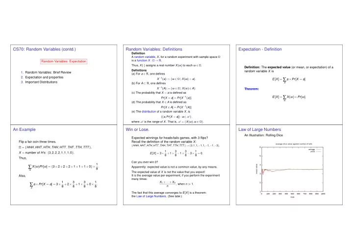
CS70: Random Variables (contd.) Random Variables: Definitions Expectation - Definition Definition A random variable, X , for a random experiment with sample space Ω is a function X : Ω → ℜ . Random Variables: Expectation Thus, X ( · ) assigns a real number X ( ω ) to each ω ∈ Ω . Definition: The expected value (or mean, or expectation) of a Definitions random variable X is 1. Random Variables: Brief Review (a) For a ∈ ℜ , one defines 2. Expectation and properties E [ X ] = ∑ X − 1 ( a ) := { ω ∈ Ω | X ( ω ) = a } . a × Pr [ X = a ] . 3. Important Distributions a (b) For A ⊂ ℜ , one defines X − 1 ( A ) := { ω ∈ Ω | X ( ω ) ∈ A } . Theorem: (c) The probability that X = a is defined as E [ X ] = ∑ X ( ω ) × Pr [ ω ] . Pr [ X = a ] = Pr [ X − 1 ( a )] . ω (d) The probability that X ∈ A is defined as Pr [ X ∈ A ] = Pr [ X − 1 ( A )] . (e) The distribution of a random variable X , is { ( a , Pr [ X = a ]) : a ∈ A } , where A is the range of X . That is, A = { X ( ω ) , ω ∈ Ω } . An Example Win or Lose. Law of Large Numbers An Illustration: Rolling Dice Expected winnings for heads/tails games, with 3 flips? Flip a fair coin three times. Recall the definition of the random variable X : { HHH , HHT , HTH , HTT , THH , THT , TTH , TTT } → { 3 , 1 , 1 , − 1 , 1 , − 1 , − 1 , − 3 } . Ω = { HHH , HHT , HTH , THH , HTT , THT , TTH , TTT } . E [ X ] = 3 × 1 8 + 1 × 3 8 − 1 × 3 8 − 3 × 1 X = number of H ’s: { 3 , 2 , 2 , 2 , 1 , 1 , 1 , 0 } . 8 = 0 . Thus, Can you ever win 0? X ( ω ) Pr [ ω ] = { 3 + 2 + 2 + 2 + 1 + 1 + 1 + 0 }× 1 ∑ 8 . Apparently: expected value is not a common value, by any means. ω The expected value of X is not the value that you expect! It is the average value per experiment, if you perform the experiment Also, many times: a × Pr [ X = a ] = 3 × 1 8 + 2 × 3 8 + 1 × 3 8 + 0 × 1 X 1 + ··· + X n ∑ , when n ≫ 1 . 8 . n a The fact that this average converges to E [ X ] is a theorem: the Law of Large Numbers. (See later.)
Indicators Linearity of Expectation Using Linearity - 1: Pips (dots) on dice Definition Theorem: Expectation is linear Roll a die n times. Let A be an event. The random variable X defined by X m = number of pips on roll m . E [ a 1 X 1 + ··· + a n X n ] = a 1 E [ X 1 ]+ ··· + a n E [ X n ] . � 1 , if ω ∈ A X = X 1 + ··· + X n = total number of pips in n rolls. X ( ω ) = 0 , if ω / ∈ A Proof: E [ X ] = E [ X 1 + ··· + X n ] is called the indicator of the event A . = E [ X 1 ]+ ··· + E [ X n ] , by linearity E [ a 1 X 1 + ··· + a n X n ] = ∑ = nE [ X 1 ] , because the X m have the same distribution ( a 1 X 1 + ··· + a n X n )( ω ) Pr [ ω ] Note that Pr [ X = 1 ] = Pr [ A ] and Pr [ X = 0 ] = 1 − Pr [ A ] . ω Hence, = ∑ Now, ( a 1 X 1 ( ω )+ ··· + a n X n ( ω )) Pr [ ω ] E [ X 1 ] = 1 × 1 6 + ··· + 6 × 1 6 = 6 × 7 × 1 6 = 7 ω 2 . E [ X ] = 1 × Pr [ X = 1 ]+ 0 × Pr [ X = 0 ] = Pr [ A ] . 2 = a 1 ∑ X 1 ( ω ) Pr [ ω ]+ ··· + a n ∑ X n ( ω ) Pr [ ω ] ω ω This random variable X ( ω ) is sometimes written as = a 1 E [ X 1 ]+ ··· + a n E [ X n ] . Hence, E [ X ] = 7 n 2 . 1 { ω ∈ A } or 1 A ( ω ) . Note: If we had defined Y = a 1 X 1 + ··· + a n X n has had tried to Note: Computing ∑ x xPr [ X = x ] directly is not easy! compute E [ Y ] = ∑ y yPr [ Y = y ] , we would have been in trouble! Thus, we will write X = 1 A . Using Linearity - 2: Random assignments Example Using Linearity - 3: Binomial Distribution. Calculating E [ g ( X )] Let Y = g ( X ) . Assume that we know the distribution of X . Flip n coins with heads probability p . X - number of heads Hand out assignments at random to n students. We want to calculate E [ Y ] . Binomial Distibution: Pr [ X = i ] , for each i . X = number of students that get their own assignment back. Method 1: We calculate the distribution of Y : X = X 1 + ··· + X n where � n � p i ( 1 − p ) n − i . Pr [ Y = y ] = Pr [ X ∈ g − 1 ( y )] where g − 1 ( x ) = { x ∈ ℜ : g ( x ) = y } . Pr [ X = i ] = X m = 1 { student m gets his/her own assignment back } . i One has This is typically rather tedious! � n � E [ X ] = ∑ i × Pr [ X = i ] = ∑ p i ( 1 − p ) n − i . Method 2: We use the following result. i × E [ X ] = E [ X 1 + ··· + X n ] i i i = E [ X 1 ]+ ··· + E [ X n ] , by linearity Theorem: E [ g ( X )] = ∑ g ( x ) Pr [ X = x ] . Uh oh. ... Or... a better approach: Let = nE [ X 1 ] , because all the X m have the same distribution x � 1 Proof: = nPr [ X 1 = 1 ] , because X 1 is an indicator if i th flip is heads X i = = ∑ g ( X ( ω )) Pr [ ω ] = ∑ ∑ = n ( 1 / n ) , because student 1 is equally likely E [ g ( X )] g ( X ( ω )) Pr [ ω ] 0 otherwise x ω ω ∈ X − 1 ( x ) to get any one of the n assignments E [ X i ] = 1 × Pr [“ heads ′′ ]+ 0 × Pr [“ tails ′′ ] = p . = ∑ g ( x ) Pr [ ω ] = ∑ ∑ ∑ g ( x ) Pr [ ω ] = 1 . x x ω ∈ X − 1 ( x ) ω ∈ X − 1 ( x ) Note that linearity holds even though the X m are not independent. Moreover X = X 1 + ··· X n and = ∑ g ( x ) Pr [ X = x ] . Note: What is Pr [ X = m ] ? Tricky .... E [ X ] = E [ X 1 ]+ E [ X 2 ]+ ··· E [ X n ] = n × E [ X i ]= np . x
µ X ⇔ µ X An Example Center of Mass Monotonicity Let X be uniform in {− 2 , − 1 , 0 , 1 , 2 , 3 } . Definition Let also g ( X ) = X 2 . Then (method 2) The expected value has a center of mass interpretation: Let X , Y be two random variables on Ω . We write X ≤ Y if X ( ω ) ≤ Y ( ω ) for all ω ∈ Ω , and similarly for X ≥ Y and X ≥ a 0 . 5 0 . 5 0 . 7 0 . 3 for some constant a . 3 x 2 1 ∑ E [ g ( X )] = Facts 6 0 1 0 1 x = − 2 0 . 7 (a) If X ≥ 0, then E [ X ] ≥ 0. 0 . 5 { 4 + 1 + 0 + 1 + 4 + 9 } 1 6 = 19 (b) If X ≤ Y , then E [ X ] ≤ E [ Y ] . = 6 . p 1 p 2 p 3 p n ( a n − µ ) = 0 Proof Method 1 - We find the distribution of Y = X 2 : a 2 a 3 n (a) If X ≥ 0 , every value a of X is nonnegative. Hence, a 1 = a n p n = E [ X ] w.p. 2 4 , p 1 ( a 1 − µ ) n E [ X ] = ∑ p 3 ( a 3 − µ ) aPr [ X = a ] ≥ 0 . 6 p 2 ( a 2 − µ ) w.p. 2 1 , a 6 Y = w.p. 1 0 , 6 w.p. 1 9 , 6 . (b) X ≤ Y ⇒ Y − X ≥ 0 ⇒ E [ Y ] − E [ X ] = E [ Y − X ] ≥ 0 . Example: Thus, E [ Y ] = 42 6 + 12 6 + 01 6 + 91 6 = 19 B = ∪ m A m ⇒ 1 B ( ω ) ≤ ∑ m 1 A m ( ω ) ⇒ Pr [ ∪ m A m ] ≤ ∑ m Pr [ A m ] . 6 . Summary Random Variables ◮ A random variable X is a function X : Ω → ℜ . ◮ Pr [ X = a ] := Pr [ X − 1 ( a )] = Pr [ { ω | X ( ω ) = a } ] . ◮ Pr [ X ∈ A ] := Pr [ X − 1 ( A )] . ◮ The distribution of X is the list of possible values and their probability: { ( a , Pr [ X = a ]) , a ∈ A } . ◮ E [ X ] := ∑ a aPr [ X = a ] . ◮ Expectation is Linear.
Recommend
More recommend
Explore More Topics
Stay informed with curated content and fresh updates.

