Dynamic Region-biased Rapidly-exploring Random Trees by Jory - PowerPoint PPT Presentation
Dynamic Region-biased Rapidly-exploring Random Trees by Jory Denny, Read Sandstrom, Andrew Bregger, and Nancy M. Amato University of Richmond, Richmond VA, USA Texas A&M University, College Station, TX, USA Presenter: Jae Won Choi RRT
Dynamic Region-biased Rapidly-exploring Random Trees by Jory Denny, Read Sandstrom, Andrew Bregger, and Nancy M. Amato University of Richmond, Richmond VA, USA Texas A&M University, College Station, TX, USA Presenter: Jae Won Choi
RRT Review
RRT Review • RRT - Randomized Sampling
RRT Review • RRT - Randomized Sampling
RRT Review • RRT - Randomized Sampling
RRT Review • RRT - Randomized Sampling
RRT Review • RRT - Randomized Sampling
RRT Review • RRT - Randomized Sampling
RRT Review • RRT - Randomized Sampling
RRT Review • RRT - Randomized Sampling
RRT Review • RRT - Randomized Sampling
RRT Review • RRT - Randomized Sampling + Simple way to construct an approximate model of problem space
RRT Review • RRT - Randomized Sampling + Simple way to construct an approximate model of problem space - Weak with narrow and cluttered spaces
Related Work 1 • Dynamic Domain RRT + Reduces unnecessary samples from boundary regions + High probability of sampling narrow passage - Worst case same as Regular RRT (a)Regular RRT sampling domain (b)Visible Voronoi region (c)Dynamic Domain Dynamic-Domain RRTs: Efficient Exploration by Controlling the Sampling Domain by Yershova, Jaillet, Simeon, and La Valle.
Related Work 2 • Obstacle-based RRT (OBRRT) : • Growing tree based on obstacle hints 1. Choose a node to grow from – G0: Basic Extension 2. Choose a growth method G1: Random position, Same orientation 3. Generate target configuration G2: Random obstacle vector, Random Orientation 4. Extend from source configuration G3: Random Obstacle Vector, Same toward target configuration Orientation G4: Rotation followed by Extension G5: … G6: … … G9 An Obstacle-Based Rapidly-Exploring Random Tree by Samuel Rodriguez, Xinyu Tang, Jyh-Ming Lien and Nancy M. Amato
Related Work 3 • Retraction-based RRT + Improve performance of RRT in narrow passages by sampling near the boundary of C-obstacle - Slower than Regular RRT when there are no narrow passages An Efficient Retration-based RRT Planner by Liangjun Zhang and Dinesh Manocha
Related Work 4 • RRT* • Tree locally rewires itself to ensure optimization of a cost function + Effective in finding shortest path - In practice, it requires many iterations to produce near optimal solutions (a) 500, (b) 1500, (c) 2500, (d) 5000, (e) 10,000, (f) 15,000 iterations
More Related Works • RRT-Blossom • Stable Sparse-RRT …
Dynamic Region RRT Input : Environment e and a query (q s , q g ) 1. G <- Compute Embedding Graph(e) [pre computation] 2. F <- Compute Flow Graph (G, q s , q g ) 3. R <- Initialize Regions (F, q s ) 4. While not done do 5. Region Biased RRT Growth (F, R)
Dynamic Region RRT Input : Environment e and a query (q s , q g ) 1. G <- Compute Embedding Graph(e) [pre computation] 2. F <- Compute Flow Graph (G, q s , q g ) 3. R <- Initialize Regions (F, q s ) 4. While not done do 5. Region Biased RRT Growth (F, R)
Dynamic Region RRT Input : Environment e and a query (q s , q g ) 1. G <- Compute Embedding Graph(e) [pre computation] 2. F <- Compute Flow Graph (G, q s , q g ) 3. R <- Initialize Regions (F, q s ) 4. While not done do 5. Region Biased RRT Growth (F, R)
Dynamic Region RRT Input : Environment e and a query (q s , q g ) 1. G <- Compute Embedding Graph(e) [pre computation] 2. F <- Compute Flow Graph (G, q s , q g ) 3. R <- Initialize Regions (F, q s ) 4. While not done do 5. Region Biased RRT Growth (F, R)
Dynamic Region RRT Input : Environment e and a query (q s , q g ) 1. G <- Compute Embedding Graph(e) [pre computation] 2. F <- Compute Flow Graph (G, q s , q g ) 3. R <- Initialize Regions (F, q s ) 4. While not done do 5. Region Biased RRT Growth (F, R)
1. Embedding Graph • Computing Embedding Graph
1. Embedding Graph • Computing Embedding Graph Generalized Voronoi Graph
1. Embedding Graph • Computing Embedding Graph 1. Compute Tetrahedralization of the environment
1. Embedding Graph • Computing Embedding Graph 1. Compute Tetrahedralization of the environment 2. Construct a Reeb Graph from the Tetrahedralization
1. Embedding Graph • Computing Embedding Graph 1. Compute Tetrahedralization of the environment 2. Construct a Reeb Graph from the Tetrahedralization F = z coordinate of a point on manifold M Maximum Saddle Minimum
F = y coordinate of a point 1. Embedding Graph on manifold M • Computing Embedding Graph 1. Compute Tetrahedralization of the environment 2. Construct a Reeb Graph from the Tetrahedralization F = z coordinate of a point on manifold M Maximum Saddle Minimum 2 Minimums Saddle Saddle Saddle Saddle 2 Maximums
1. Embedding Graph • Computing Embedding Graph 1. Compute Tetrahedralization of the environment 2. Construct a Reeb Graph from the Tetrahedralization F = z coordinate of a point on manifold M Maximum Saddle Minimum
1. Embedding Graph • Computing Embedding Graph 1. Compute Tetrahedralization of the environment 2. Construct a Reeb Graph from the Tetrahedralization 3. Embed the Reeb graph back to the Environment
1. Embedding Graph • Computing Embedding Graph 1. Compute Tetrahedralization of the environment 2. Construct a Reeb Graph from the Tetrahedralization 3. Embed the Reeb graph back to the Environment Naïve Reeb Graph Algorithm: O(n 2 )
1. Embedding Graph • Computing Embedding Graph 1. Compute Tetrahedralization of the environment 2. Construct a Reeb Graph from the Tetrahedralization 3. Embed the Reeb graph back to the Environment Naïve Reeb Graph Algorithm: O(n 2 ) Fast Reeb Graph Algorithm: O(n log(n))
2. Flow Graph • Computing Flow Graph
2. Flow Graph • Computing Flow Graph 1. Perform BFS from the nearest node q s
2. Flow Graph • Computing Flow Graph 1. Perform BFS from the nearest node q s
2. Flow Graph • Computing Flow Graph 1. Perform BFS from the nearest node q s
2. Flow Graph • Computing Flow Graph 1. Perform BFS from the nearest node q s 2. Backtrack from the nearest node to q g to trim unrelated edges to a solution path (pruning)
2. Flow Graph • Computing Flow Graph 1. Perform BFS from the nearest node q s 2. Backtrack from the nearest node to q g to trim unrelated edges to a solution path (pruning)
2. Flow Graph • Computing Flow Graph 1. Perform BFS from the nearest node q s 2. Backtrack from the nearest node to q g to trim unrelated edges to a solution path (pruning)
2. Flow Graph • Computing Flow Graph 1. Perform BFS from the nearest node q s 2. Backtrack from the nearest node to q g to trim unrelated edges to a solution path (pruning)
3. Region-biased RRT Growth • Four steps
3. Region-biased RRT Growth • Four steps 1. Region-biased RRT extension * Samples the region for a and then performs like any RRT method
3. Region-biased RRT Growth • Four steps 1. Region-biased RRT extension * Samples the region for a and then performs like any RRT method 2. Advance regions along flow edges
3. Region-biased RRT Growth • Four steps 1. Region-biased RRT extension * Samples the region for a and then performs like any RRT method 2. Advance regions along flow edges 3. Delete useless regions(heuristic) 4. Create new regions
3. Region-biased RRT Growth • Four steps 1. Region-biased RRT extension * Samples the region for a and then performs like any RRT method 2. Advance regions along flow edges 3. Delete useless regions(heuristic) 4. Create new regions
Evaluation
Results on Holonomic
Results on non-holonomic + Dynamic biased RRT works on non-holonomic problems - SyClop performs better * SyClop has faster neighbor selection routine
Results
Q&A
Recommend
More recommend
Explore More Topics
Stay informed with curated content and fresh updates.

