Dummy Endogenous Variables in a Simultaneous Equation System - PowerPoint PPT Presentation
Dummy Endogenous Variables in a Simultaneous Equation System Econometrica, Vol. 46, No. 4 (Jul., 1978), 931-959. James J. Heckman Econ 312, Spring 2019 Heckman 5/29/2019 1. A GENERAL MODEL FOR THE TWO EQUATION CASE Heckman Dummy Endogenous
Dummy Endogenous Variables in a Simultaneous Equation System Econometrica, Vol. 46, No. 4 (Jul., 1978), 931-959. James J. Heckman Econ 312, Spring 2019 Heckman 5/29/2019
1. A GENERAL MODEL FOR THE TWO EQUATION CASE Heckman Dummy Endogenous Variables
∗ and y 2i ∗ , • Pair of simultaneous equations for continuous latent random variables 𝑧 1𝑗 ∗ = 𝑌 1𝑗 𝛽 1 + 𝑒 𝑗 𝛾 1 + 𝑧 2𝑗 ∗ 𝜇 1 + 𝑉 1𝑗 , (1a) 𝑧 1𝑗 ∗ = 𝑌 2𝑗 𝛽 2 + 𝑒 𝑗 𝛾 2 + 𝑧 1𝑗 ∗ 𝜇 2 + 𝑉 2𝑗 , (2a) 𝑧 2𝑗 where dummy variable 𝑒 𝑗 is defined by ∗ > 0 , (1c) 𝑒 𝑗 = 1 iff 𝑧 2𝑗 𝑒 𝑗 = 0 otherwise, and 2 = 𝜏 𝐹 𝑉 𝑘𝑗 = 0, 𝐹 𝑉 𝑘𝑘 , 𝐹 𝑉 1𝑗 𝑉 2𝑗 = 𝜏 12 , 𝑘 = 1,2; 𝑗 = 1, … , 𝐽. 𝑘𝑗 𝑘𝑗 𝑉 𝑘 ′ 𝑗 ′ = 0, for 𝑘, 𝑘 ′ = 1,2; 𝑗 ≠ 𝑗 ′ . 𝐹 𝑉 “ 𝑌 1𝑗 ” and “ 𝑌 2𝑗 ” are, respectively, 1 × 𝐿 1 and 1 × 𝐿 2 row vectors of bounded exogenous variables. Heckman Dummy Endogenous Variables
• Equations (1a) and (1b) are identified under standard conditions if 𝛾 1 = 𝛾 2 = ∗ and 𝑧 2𝑗 ∗ are observed for each of the I observations. 0 and both 𝑧 1𝑗 • In this special case, which conforms to the classical simultaneous equation model, standard methods are available to estimate all of the parameters of the structure. ∗ and 𝑧 2𝑗 ∗ which • First, note that the model is cast in terms of latent variables 𝑧 1𝑗 may or may not be directly observed. ∗ is never observed, the event 𝑧 2𝑗 ∗ > 0 is observed and its occurrence • Even if 𝑧 2𝑗 is recorded by setting a dummy variable, 𝑒 𝑗 equal to one. ∗ < 0, the dummy variable assumes the value zero. • If 𝑧 2𝑗 ∗ > 0, structural equations (1a) and (1b) are shifted by an • Second, note that if 𝑧 2𝑗 amount 𝛾 1 and 𝛾 2 , respectively. Heckman Dummy Endogenous Variables
• To fix ideas, several plausible economic models are discussed that may be described by equation system (1a)-(1c). ∗ and 𝑧 2𝑗 ∗ are observed outcomes of a market at • First, suppose that both 𝑧 1𝑗 time i, say quantity and price. • Equation (1a) is the demand curve while equation (1b) is the supply curve. • If the price exceeds some threshold (zero in inequality (1c), but this can be readily amended t be any positive constant), the government takes certain actions that shift both the supply curve and the demand curve, say a subsidy to consumers and a per unit subsidy to producers. • These actions shift the demand curve and the supply curve by the amount 𝛾 1 and 𝛾 2 , respectively. Heckman Dummy Endogenous Variables
• As another example, consider a model of the effect of laws on the status of blacks. ∗ be the measured income of blacks in state i while 𝑧 2𝑗 ∗ is an • Let 𝑧 1𝑗 unmeasured variable that reflects the state’s population sentiment toward blacks. ∗ > 0 the state may • If sentiment for blacks is sufficiently favorable 𝑧 2𝑗 enact antidiscrimination legislation and the presence of such legislation in state i , a variable that can be measured, is denoted by a dummy variable 𝑒 𝑗 = 1 . • In the income equation (1a), both the presence of a law and the population sentiment towards blacks is assumed to affect the measured income of blacks. • The first effect is assumed to operate discretely while the second effect is assumed to operate in a more continuous fashion. Heckman Dummy Endogenous Variables
• Two conceptually distinct roles for dummy variables: 1. As indicators of latent variables that cross thresholds and 2. As direct shifters of behavioral functions. These two roles must be carefully distinguished. Heckman Dummy Endogenous Variables
• The model of equations (1a)-(1c) subsumes a wide variety of interesting econometric models. These special cases are briefly discussed in turn. • CASE l: The Classical Simultaneous Equation Model: This model ∗ and 𝑧 2𝑗 ∗ are observed, and there is no structural shift arises when 𝑧 1𝑗 in the equations (𝛾 1 = 𝛾 2 = 0) . • CASE 2: The Classical Simultaneous Equation Model with Structural Shift: This model is the same as that of Case 1 except that structural shift is permitted in each equation. It will be shown below that certain restrictions must be imposed on the model in order to generate a sensible statistical structure for this case. Heckman Dummy Endogenous Variables
• CASE 3: The Multivariate Probit Model: This model arises when ∗ and 𝑧 2𝑗 ∗ are not observed but the events 𝑧 1𝑗 ∗ and 𝑧 2𝑗 ∗ are observed 𝑧 1𝑗 (i.e., one knows whether or not the latent variables have crossed a threshold). The notation of equations (1a)-(1b) must be altered to accommodate two dummy variables but that modification is obvious. No structural shift is permitted ( 𝛾 1 = 𝛾 2 = 0 ). This is the model of Ashford and Sowden [3], Amemiya [2], and Zellner and Lee [30]. • CASE 4: The Multivariate Probit Model with Structural Shift: This model is the same as that of Case 3 except that structural shift is permitted ( 𝛾 1 = 𝛾 2 = 0 ). Heckman Dummy Endogenous Variables
∗ is • CASE 5: The Hybrid Model: This model arises when 𝑧 1𝑗 ∗ ≷ 0 is observed. No ∗ is not, but the event 𝑧 2𝑗 observed and 𝑧 2𝑗 structural shift is permitted ( 𝛾 1 = 𝛾 2 = 0 ). • CASE 6: The Hybrid Model with Structural Shift: This model is the same as that of Case 5 except that structural shifts in the equations are permitted. Heckman Dummy Endogenous Variables
2. THE HYBRID MODEL WITH STRUCTURAL SHIFT Heckman Dummy Endogenous Variables
• In this section, a model with one observed continuous random variable, and one latent random variable is analyzed for the general case of structural shift in the equations. • Consider identification only; Heckman (1978) for additional discussion. Heckman Dummy Endogenous Variables
• To facilitate the discussion, equations (1a) and (1b) may be written in semi-reduced form as Heckman Dummy Endogenous Variables
• In the ensuing analysis it is assumed that exogenous variables included in both 𝑌 1𝑗 and 𝑌 2𝑗 are allocated to either 𝑌 1𝑗 or 𝑌 2𝑗 but not both. • The absence of an asterisk on 𝑧 1𝑗 denotes that this variable is observed. ∗ ” is not observed. • “ 𝑧 2𝑗 • Random variables 𝑉 1𝑗 and 𝑉 2𝑗 are assumed to be bivariate normal random variables. • Accordingly, the joint distribution of 𝑊 1𝑗 , 𝑊 2𝑗 , ℎ(𝑊 1𝑗 , 𝑊 2𝑗 ) , is a bivariate normal density fully characterized by the following assumptions: 𝐹 𝑊 1𝑗 = 0, 𝐹 𝑊 2𝑗 = 0, 2 2 𝐹 𝑊 = 𝜕 1𝑗 , 𝐹 𝑊 1𝑗 𝑊 2𝑗 = 𝜕 12 , 𝐹 𝑊 = 𝜕 22 . 1𝑗 2𝑗 Heckman Dummy Endogenous Variables
Heckman Dummy Endogenous Variables
(i) Conditions for Existence of the Model Heckman Dummy Endogenous Variables
• The first order of business is to determine whether or not the model of equations (1a)-(1b) as represented in reduced form by equations (3a)-(3b) makes sense. • Without imposing a further restriction, it does not. • The restriction required is precisely the restriction implicitly assumed in writing equations (3a) and (3b), i.e., the restriction that permits one to define a unique probability statement for the events 𝑒 𝑗 = 1 and 𝑒 𝑗 = 0 so that 𝑄 𝑗 in fact exists. • A necessary and sufficient condition for this to be so is that 𝜌 23 = 0 , i.e., that the probability of the event 𝑒 𝑗 = 1 is not a determinant of the event. • Equivalently, this assumption can be written as the requirement that 𝛿 2 𝛾 1 + 𝛾 2 = 0 . • This condition is critical to the analysis and thus deserves some discussion. • The argument supporting this assumption is summarized in the following proposition. Heckman Dummy Endogenous Variables
PROPOSITION: A necessary and sufficient condition for the model of equations (1a)-(1c) or (3a)-(3c) to be defined is that 𝜌 23 = 0 = 𝛿 2 𝛾 1 + 𝛾 2 . This assumption is termed the principal assumption. PROOF: Sufficiency is obvious. Thus, only necessary conditions are discussed. Denote the joint density of 𝑊 2𝑗 , 𝑒 𝑗 by 𝑢(𝑊 2𝑗 , 𝑒 𝑗 ) which is assumed to be a proper density in the sense that ∞ 𝑢(𝑊 2𝑗 , 𝑒 𝑗 ) 𝑒𝑊 2𝑗 = 1. −∞ 𝑒 𝑗 =0,1 ∗ ⩾ 0 given 𝑒 𝑗 = 1 must be • From equations (3b) and (3c), the probability that 𝑧 2𝑗 unity, so that one may write Pr 𝑊 2𝑗 > 𝑚 𝑗 𝑒 𝑗 = 1 = 1 ′ = ′ are defined by 𝑚 𝑗 = − 𝑌 1𝑗 𝜌 21 + 𝑌 22 + 𝜌 23 and 𝑚 𝑗 where the symbols 𝑚 𝑗 and 𝑚 𝑗 𝑚 𝑗 + 𝜌 23 . Heckman Dummy Endogenous Variables
• Alternatively, one may write this condition as ∞ 𝑢(𝑊 2𝑗 , 1) 𝑒𝑊 2𝑗 = 𝑄 𝑗 (4a) 𝑚 𝑗 and obviously 𝑚 𝑗 𝑢 𝑊 2𝑗 , 1 𝑒𝑊 2𝑗 = 0. (4b) −∞ • Using similar reasoning, one can conclude that ′ 𝑚 𝑗 𝑢 𝑊 2𝑗 , 1 𝑒𝑊 2𝑗 = 1 − 𝑄 𝑗 (4c) −∞ and ∞ 𝑢 𝑊 2𝑗 , 0 𝑒𝑊 2𝑗 = 0. (4d) ′ 𝑚 𝑗 Heckman Dummy Endogenous Variables
Recommend
More recommend
Explore More Topics
Stay informed with curated content and fresh updates.
