Draft Static Network Reliability Estimation Under the - PowerPoint PPT Presentation

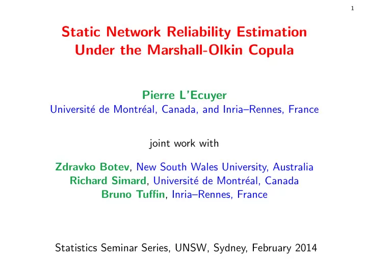
1 Draft Static Network Reliability Estimation Under the Marshall-Olkin Copula Pierre L’Ecuyer Universit´ e de Montr´ eal, Canada, and Inria–Rennes, France joint work with Zdravko Botev , New South Wales University, Australia Richard Simard , Universit´ e de Montr´ eal, Canada Bruno Tuffin , Inria–Rennes, France Statistics Seminar Series, UNSW, Sydney, February 2014

2 Draft A static network reliability problem A system has m components, in state 0 (failed) or 1 (operating). System state: X = ( X 1 , . . . , X m ) t . Structure function: Φ : { 0 , 1 } m → { 0 , 1 } , assumed monotone. System is operational iff Φ( X ) = 1. Unreliability: u = P [Φ( X ) = 0].

2 Draft A static network reliability problem A system has m components, in state 0 (failed) or 1 (operating). System state: X = ( X 1 , . . . , X m ) t . Structure function: Φ : { 0 , 1 } m → { 0 , 1 } , assumed monotone. System is operational iff Φ( X ) = 1. Unreliability: u = P [Φ( X ) = 0]. If we know p ( x ) = P [ X = x ] for all x ∈ { 0 , 1 } m , in theory we can compute � u = p ( x ) . x ∈D = { X :Φ( X )=0 } But the cost of enumerating D is generally exponential in m . The X i ’s may be dependent.

3 Draft Monte Carlo (MC): Generate n i.i.d. realizations of X , say X 1 , . . . , X n , compute W i = Φ( X i ) for each i , and estimate u by ¯ W n = ( W 1 + · · · + W n ) / n ∼ Binomial ( n , u ) / n ≈ Poisson ( nu ) / n . Can also estimate Var [ ¯ W n ] and compute a confidence interval on u .

3 Draft Monte Carlo (MC): Generate n i.i.d. realizations of X , say X 1 , . . . , X n , compute W i = Φ( X i ) for each i , and estimate u by ¯ W n = ( W 1 + · · · + W n ) / n ∼ Binomial ( n , u ) / n ≈ Poisson ( nu ) / n . Can also estimate Var [ ¯ W n ] and compute a confidence interval on u . When u is very small (failure is a rare event), direct MC fails. Ex: if u = 10 − 10 , system fails once per 10 billion runs on average.

3 Draft Monte Carlo (MC): Generate n i.i.d. realizations of X , say X 1 , . . . , X n , compute W i = Φ( X i ) for each i , and estimate u by ¯ W n = ( W 1 + · · · + W n ) / n ∼ Binomial ( n , u ) / n ≈ Poisson ( nu ) / n . Can also estimate Var [ ¯ W n ] and compute a confidence interval on u . When u is very small (failure is a rare event), direct MC fails. Ex: if u = 10 − 10 , system fails once per 10 billion runs on average. Relative error √ 1 − u MSE [ ¯ � W n ] W n ] def here RE [ ¯ = = √ nu → ∞ when u → 0 . u For example, if u ≈ 10 − 10 , we need n ≈ 10 12 to have RE [ ¯ W n ] ≤ 10%. We would like bounded RE (or almost) when u → 0.

4 Draft Although our methods apply much more generally, we focus here on the case where Φ is defined by a graph. Link i “works” iff X i = 1. The system is operational iff all the nodes in a given set V 0 are connected. X 11 6 9 X 6 X 10 X 13 3 X 2 X 5 5 8 X 9 X 3 1 X 8 X 12 X 1 2 4 7 X 4 X 7 Given X , Φ( X ) is easy to evaluate by graph algorithms (e.g., minimal spanning tree). Challenge: How to sample X effectively. We propose methods based on (a) conditional MC and (b) splitting .

5 Draft Conditional MC with auxiliary variables [Elperin, Gertsbach, Lomonosov 1974, 1991, 1992, etc.] Special case: the X i ’s are independent with P [ X i = 0] = u i . Conceptually, suppose each link i is initially failed and gets repaired at time Y i ∼ Expon( µ i ) where µ i = − ln( u i ). Then P [ Y i > 1] = P [ X i = 0] = u i . Let Y = ( Y 1 , . . . , Y m ) and π the permutation s.t. Y π (1) < · · · < Y π ( m ) . Conditional on π , we can forget the Y i ’s, add the (non-redundant) links one by one until the graph is operational, say at step C . Data structure: forest of spanning trees. Adding a link may merge two trees.

5 Draft Conditional MC with auxiliary variables [Elperin, Gertsbach, Lomonosov 1974, 1991, 1992, etc.] Special case: the X i ’s are independent with P [ X i = 0] = u i . Conceptually, suppose each link i is initially failed and gets repaired at time Y i ∼ Expon( µ i ) where µ i = − ln( u i ). Then P [ Y i > 1] = P [ X i = 0] = u i . Let Y = ( Y 1 , . . . , Y m ) and π the permutation s.t. Y π (1) < · · · < Y π ( m ) . Conditional on π , we can forget the Y i ’s, add the (non-redundant) links one by one until the graph is operational, say at step C . Data structure: forest of spanning trees. Adding a link may merge two trees. Permutation Monte Carlo (PMC) estimator: conditional probability that the total time for these repairs is larger than 1: P [ A 1 + · · · + A c > 1 | π, C = c ] . At step j , the time A j to next repair is exponential with rate Λ j , the sum of repair rates of all links not yet repaired. Sum is an hypoexponential. Theorem [Gertsback and Shpungin 2010]. Gives BRE when the u i → 0.

5 Draft Conditional MC with auxiliary variables [Elperin, Gertsbach, Lomonosov 1974, 1991, 1992, etc.] Special case: the X i ’s are independent with P [ X i = 0] = u i . Conceptually, suppose each link i is initially failed and gets repaired at time Y i ∼ Expon( µ i ) where µ i = − ln( u i ). Then P [ Y i > 1] = P [ X i = 0] = u i . Let Y = ( Y 1 , . . . , Y m ) and π the permutation s.t. Y π (1) < · · · < Y π ( m ) . Conditional on π , we can forget the Y i ’s, add the (non-redundant) links one by one until the graph is operational, say at step C . Data structure: forest of spanning trees. Adding a link may merge two trees. Permutation Monte Carlo (PMC) estimator: conditional probability that the total time for these repairs is larger than 1: P [ A 1 + · · · + A c > 1 | π, C = c ] . At step j , the time A j to next repair is exponential with rate Λ j , the sum of repair rates of all links not yet repaired. Sum is an hypoexponential. Theorem [Gertsback and Shpungin 2010]. Gives BRE when the u i → 0. Improvement: turnip ; at each step, discard redundant unrepaired links.

6 Draft We have c c Λ k � � e − Λ j P [ A 1 + · · · + A c > 1 | π, C = c ] = . Λ k − Λ j j =1 k =1 , k � = j This formula becomes unstable when c is large and/or the Λ j are small. The product terms are very large and have alternate signs ( − 1) j − 1 . Higham (2009) propose a stable method for matrix exponential. More reliable, but significantly slower.

6 Draft We have c c Λ k � � e − Λ j P [ A 1 + · · · + A c > 1 | π, C = c ] = . Λ k − Λ j j =1 k =1 , k � = j This formula becomes unstable when c is large and/or the Λ j are small. The product terms are very large and have alternate signs ( − 1) j − 1 . Higham (2009) propose a stable method for matrix exponential. More reliable, but significantly slower. For the case where the above prob is close to 1, we also have c c Λ k � (1 − e − Λ j ) � P [ A 1 + · · · + A c ≤ 1 | π, C = c ] = . Λ k − Λ j j =1 k =1 , k � = j

7 Draft A dodecahedron network B 28 27 20 18 11 25 19 30 29 10 9 4 3 1 8 5 17 12 26 21 A 16 2 13 7 6 15 14 24 22 23

8 Draft Turnip method for dodecahedron graph: n = 10 6 , V 0 = { 1 , 20 } 10 − 1 10 − 2 10 − 3 10 − 4 10 − 5 10 − 6 u i = ǫ ¯ W 2.881e-3 2.065e-6 2.006e-9 1.992e-12 1.999e-15 2.005e-18 n RE[ ¯ W n ] 0.00302 0.00421 0.00433 0.00436 0.00435 0.00434 T (sec) 15.6 15.5 15.5 15.5 15.5 15.5 We see that u ≈ 2 × 10 − 3 ǫ and RE is bounded (proved).

9 Draft Three dodecahedron graphs in parallel. 60 nodes and 90 links. dodec. 2 A dodec. 1 B dodec. 3

10 Draft Turnip for three dodecahedrons in parallel: n = 10 8 , V 0 = { 1 , 20 } 10 − 1 10 − 2 10 − 3 10 − 4 10 − 5 10 − 6 u i = ǫ ¯ W 2.39e-8 8.80e-18 8.20e-27 8.34e-36 8.07e-45 7.92e-54 n RE[ ¯ W n ] 0.0074 0.0194 0.0211 0.0210 0.0212 0.0215 T (sec) 6236 6227 6229 6546 6408 6289 We have u ≈ 2 × 10 − 9 ǫ and RE is bounded (proved). Total CPU time is about 2 hours, regardless of ǫ . However, for very large graphs (thousands of links), the turnip method fails, because the important permutations π , for which the conditional probability contributes significantly, are rare, and hitting them becomes a rare event. BRE does not hold for an asymptotic regime where the size of the graph increases. Splitting will come to the rescue (later on).

11 Draft Dependent Links: A Marshall-Olkin Copula Model Goal : Define a model where the X i ’s may have positive dependence.

11 Draft Dependent Links: A Marshall-Olkin Copula Model Goal : Define a model where the X i ’s may have positive dependence. We use an auxiliary dynamic model to specify the dependence. Suppose all links are initially operational. For each s ⊆ { 1 , . . . , m } , a shock that takes down all links in s occurs at an exponential time with rate λ s . Let L = { s : λ s > 0 } = { s (1) , . . . , s ( κ ) } . Denote λ j = λ s ( j ) , let Y j be the shock time for subset s ( j ), and Y = ( Y 1 , . . . , Y κ ) (the latent state of the system). X i is the the indicator that component i is operational at time 1: X i = I [ Y j > 1 for all shocks j such that i ∈ s ( j ) } .