Distribution of Eigenvalues of Linear Stochastic Systems S A DHIKARI - PowerPoint PPT Presentation
Distribution of Eigenvalues of Linear Stochastic Systems S A DHIKARI and R. S. L ANGLEY Department of Aerospace Engineering, University of Bristol, Bristol, U.K. Email: S.Adhikari@bristol.ac.uk URL:
Distribution of Eigenvalues of Linear Stochastic Systems S A DHIKARI † and R. S. L ANGLEY ‡ † Department of Aerospace Engineering, University of Bristol, Bristol, U.K. Email: S.Adhikari@bristol.ac.uk URL: http://www.aer.bris.ac.uk/contact/academic/adhikari/home.html ‡ Department of Engineering, University of Cambridge, Cambridge, UK Random Eigenvalue Problems – p.1/28
Outline of the talk • Random eigenvalue problem • Perturbation Methods • Mean-centered perturbation method • α -centered perturbation method • Asymptotic analysis • PDF of the eigenvalues • Numerical Example • Conclusions & Open Problems Random Eigenvalue Problems – p.2/28
Random eigenvalue problem The random eigenvalue problem of undamped or proportionally damped linear systems: K ( x ) φ j = λ j M ( x ) φ j (1) λ j eigenvalues; φ j eigenvectors; M ( x ) ∈ R N × N mass matrix and K ( x ) ∈ R N × N stiffness matrix. x ∈ R m is random parameter vector with pdf p ( x ) = (2 π ) − m/ 2 e − x T x / 2 (2) Random Eigenvalue Problems – p.3/28
The fundamental aim • To obtain the joint probability density function of the eigenvalues and the eigenvectors. • If the matrix M − 1 K is GUE (Gaussian unitary ensemble) or GOE (Gaussian orthogonal ensemble) an exact closed-form expression can be obtained for the joint pdf of the eigenvalues. • In general the system matrices for real structures are not GUE or GOE. Random Eigenvalue Problems – p.4/28
Mean-centered perturbation Assume that M ( 0 ) = M 0 and K ( 0 ) = K 0 are ‘deterministic parts’. Deterministic eigenvalue problem: K 0 φ j 0 = λ j 0 M 0 φ j 0 . The eigenvalues λ j ( x ) : R m → R are non-linear functions of x . Expanding λ j ( x ) by Taylor series about x = 0 : λ j ( 0 ) x + 1 x T D λ j ( 0 ) x λ j ( x ) ≈ λ j ( 0 ) + d T (3) 2 d λ j ( 0 ) ∈ R m : gradient vector, D λ j ( 0 ) ∈ R m × m the Hessian matrix of λ j ( x ) evaluated at x = 0 . Random Eigenvalue Problems – p.5/28
α -centered perturbation We are looking for a point x = α in the x -space such that the Taylor series expansion of λ j ( x ) about this point λ j ( x ) ≈ λ j ( α ) + d T λ j ( α ) ( x − α ) + 1 2 ( x − α ) T D λ j ( α ) ( x − α ) (4) is optimal in some sense. The optimal point α is selected such that the mean or the first moment of each eigenvalue is calculated most accurately. Random Eigenvalue Problems – p.6/28
α -centered perturbation The mean of λ j ( x ) can be obtained as � � m e − h ( x ) d x ¯ m λ j ( x ) p ( x ) d x = (2 π ) − m/ 2 λ j = R R (5) h ( x ) = x T x / 2 − ln λ j ( x ) where (6) Expand the function h ( x ) in a Taylor series about a point where h ( x ) attends its global minimum. By doing so the error in evaluating the integral (5) would be minimized. Random Eigenvalue Problems – p.7/28
α -centered perturbation Therefore, the optimal point can be obtained as ∂h ( x ) ∂λ j ( x ) 1 = 0 or x k = , ∀ k (7) λ j ( x ) ∂x k ∂x k Combining for all k we have d λ j ( α ) = λ j ( α ) α . Rearranging α = d λ j ( α ) /λ j ( α ) (8) This equation immediately gives a recipe for an iterative algorithm to obtain α . Random Eigenvalue Problems – p.8/28
α -centered perturbation Substituting d λ j ( α ) in Eq. (4) � 1 − | α | 2 � + 1 2 α T D λ j ( α ) α λ j ( x ) ≈ λ j ( α ) + α T � � x + 1 x T D λ j ( α ) x λ j ( α ) I − D λ j ( α ) (9) 2 This, like the mean-centered approach, also re- sults in a quadratic form in the random variable x . Random Eigenvalue Problems – p.9/28
Eigenvalue statistics Both approximations yield a quadratic form in Gaussian random variable of the form j x + 1 x T A j x λ j ( x ) ≈ c j + a T (10) 2 The moment generating function: 2 a T j [ I − s A j ] − 1 a j ≈ e sc j + s 2 � e sλ j ( x ) � M λ j ( s ) = E � (11) � I − s A j � Random Eigenvalue Problems – p.10/28
Eigenvalue statistics Cumulants: � c j + 1 2 Trace ( A j ) r = 1 , if � � κ r = a j + ( r − 1)! j A r − 2 r ! 2 a T A r Trace r ≥ 2 if j j 2 (12) Thus λ j = κ 1 = c j + 1 ¯ 2Trace ( A j ) (13) � � j a j + 1 Var [ λ j ] = κ 2 = a T A 2 2Trace (14) j Random Eigenvalue Problems – p.11/28
Asymptotic analysis We want to evaluate an integral of the following form: � � h ( x ) d x � m f ( x ) p ( x ) d x = (2 π ) − m/ 2 J = m e R R (15) h ( x ) = ln f ( x ) − x T x / 2 � where (16) Assume f ( x ) : R m → R is smooth and at least twice differentiable and � h ( x ) reaches its global maximum at an unique point θ ∈ R m . Random Eigenvalue Problems – p.12/28
Asymptotic analysis Therefore, at x = θ ∂ � h ( x ) ∂ ln f ( x ) , ∀ k, or θ = ∂ = 0 or x k = ∂ x ln f ( θ ) . ∂x k ∂x k (17) Further assume that � h ( θ ) is so large that � � � � 1 � � D j ( � h ( θ )) � → 0 for j > 2 � � (18) � � h ( θ ) D j ( � h ( θ )) : j th order derivative of � h ( x ) at x = θ . Random Eigenvalue Problems – p.13/28
Asymptotic analysis Under previous assumptions, using second-order Taylor series of � h ( x ) the integral (12) can be evaluated asymptotically as � θ � e � h ( θ ) T θ / 2 − H ( θ ) � − 1 / 2 � � J ≈ � = f ( θ ) e (19) � � H ( θ ) � H ( θ ) is the Hessian matrix of � � h ( x ) at x = θ . Random Eigenvalue Problems – p.14/28
Asymptotic analysis An arbitrary r th order moment of the eigenvalues � µ ′ m λ r j ( x ) p ( x ) d x , r = r = 1 , 2 , 3 · · · (20) R Comparing this with Eq. (12) it is clear that h ( x ) = r ln λ j ( x ) − x T x / 2 (21) � f ( x ) = λ r j ( x ) and The optimal point θ can be obtained from (14) as θ = r d λ j ( θ ) /λ j ( θ ) (22) Random Eigenvalue Problems – p.15/28
Asymptotic analysis The r th moment: � � − 1 / 2 � � j ( θ ) e − | θ | 2 � I + 1 r r θθ T − � � µ ′ r = λ r D λ j ( θ ) 2 � λ j ( θ ) (23) The mean of the eigenvalues (substitute r = 1 ): 2 � � λ j = λ j ( θ ) e − | θ | 2 � I + θθ T − D λ j ( θ ) /λ j ( θ ) � − 1 / 2 ¯ (24) Central moments: � λ j ) r � � r � = � r ( λ j − ¯ k ¯ λ r − k ( − 1) r − k µ ′ E . k =0 j k Random Eigenvalue Problems – p.16/28
Pdf of the eigenvalues Theorem 1 λ j ( x ) is distributed as a non-central χ 2 random variable with noncentrality parameter δ 2 and degrees-of-freedom m ′ if and only if (a) j = A j , (b) Trace ( A j ) = m ′ and (c) A 2 a j = A j a j , δ 2 = c j = a T j a j / 4 . This implies that the the Hessian matrix A j should be an idempotent matrix. In general this require- ment is not expected to be satisfied for eigenval- ues of real structural systems. Random Eigenvalue Problems – p.17/28
Central χ 2 approximation (Pearson’s) Pdf of the j th eigenvalue � u − � � η ) ν/ 2 − 1 e − ( u − � η ) / 2 � γ p λ j ( u ) ≈ 1 η = ( u − � γp χ 2 γ ) ν/ 2 Γ( ν/ 2) γ � � (2 � ν (25) where η = − 2 κ 22 + κ 1 κ 3 , and ν = 8 κ 23 γ = κ 3 , � � (26) κ 32 κ 3 4 κ 2 Random Eigenvalue Problems – p.18/28
Non-central χ 2 approximation Pdf of the j th eigenvalue � u − η j � p λ j ( u ) ≈ 1 p Q j (27) γ j γ j � ∞ e − ( δj + u/ 2) u m/ 2 − 1 ( δu ) r where p Q j ( u ) = r ! 2 r Γ( m/ 2+ r ) , r =0 2 m/ 2 Trace ( A j ) j A − 1 η j = c j − 1 2 a T , δ 2 j = ρ T j a j , γ j = j ρ j and 2 m ρ j = A − 1 j a j . Random Eigenvalue Problems – p.19/28
Numerical example Undamped two degree-of-system system: ¯ m 1 = 1 Kg, m 2 = 1 . 5 Kg, k 1 = 1000 ¯ k 2 = 1100 N/m and k 3 = 100 N/m. N/m, 1� 2� m� m� 1� 2� k� k� k� 2� 3� 1� Only the stiffness parameters k 1 and k 2 are uncer- k i (1 + ǫ i x i ) , i = 1 , 2 . x = { x 1 , x 2 } T ∈ R 2 tain: k i = ¯ and the ‘strength parameters’ ǫ 1 = ǫ 2 = 0 . 25 . Random Eigenvalue Problems – p.20/28
Numerical example Following six methods are compared 1. Mean-centered first-order perturbation 2. Mean-centered second-order perturbation 3. α -centered first-order perturbation 4. α -centered second-order perturbation 5. Asymptotic method 6. Monte Carlo Simulation (10K samples) - can be considered as benchmark. Random Eigenvalue Problems – p.21/28
Numerical example The percentage error: Error i th method = { µ ′ k } i th method − { µ ′ k } MCS × 100 { µ ′ k } MCS i = 1 , · · · 5 . Random Eigenvalue Problems – p.22/28
Numerical example 20 Mean−centered 1st−order Mean−centered 2nd−order 18 α −centered 1st−order α −centered 2nd−order 16 Asymptotic Method 14 Percentage error wrt MCS 12 10 8 6 4 2 0 1 2 3 4 k−th order moment: E [ λ k 1 ] Percentage error for the first four raw moments of the first eigenvalue Random Eigenvalue Problems – p.23/28
Numerical example 0 −2 −4 −6 Percentage error wrt MCS −8 −10 Mean−centered 1st−order −12 Mean−centered 2nd−order α −centered 1st−order −14 α −centered 2nd−order Asymptotic Method −16 −18 −20 1 2 3 4 k−th order moment: E [ λ k 2 ] Percentage error for the first four raw moments of the second eigenvalue Random Eigenvalue Problems – p.24/28
Recommend
More recommend
Explore More Topics
Stay informed with curated content and fresh updates.
