Discrete Dynamical Systems Computational Models for Complex Systems - PowerPoint PPT Presentation
Discrete Dynamical Systems Computational Models for Complex Systems Paolo Milazzo Dipartimento di Informatica, Universit` a di Pisa http://pages.di.unipi.it/milazzo milazzo di.unipi.it Laurea Magistrale in Informatica A.Y. 2018/2019 Paolo
Discrete Dynamical Systems Computational Models for Complex Systems Paolo Milazzo Dipartimento di Informatica, Universit` a di Pisa http://pages.di.unipi.it/milazzo milazzo di.unipi.it Laurea Magistrale in Informatica A.Y. 2018/2019 Paolo Milazzo (Universit` a di Pisa) CMCS - Discrete Dynamical Systems A.Y. 2018/2019 1 / 42
Introduction We will see how to define recurrence relations (or difference equations) in order to model the dynamics of systems whose state changes at discrete time intervals. focus on population models (birth/death of individuals) We will see that even the simplest form of interaction between individuals can lead to the emergence of complex behaviors in the population chaos! See also: Notes on a Short Course and Introduction to Dynamical Systems in Biomathematics by Urszula Fory´ s Available on the course web page Paolo Milazzo (Universit` a di Pisa) CMCS - Discrete Dynamical Systems A.Y. 2018/2019 2 / 42
Linear birth model Let N ( t ) denote the density of some population at time t . We want to construct a mathematical model able to predict the density of the same population at time t + ∆ t , that is N ( t + ∆ t ). Assume that: all individuals are the same (no dinstinction by gender, age, ...) there is enough food and space for every individual each individual has λ children every σ time units there is no death in the interval [ t , t + ∆ t ) children do not start reproducing in the interval [ t , t + ∆ t ) Paolo Milazzo (Universit` a di Pisa) CMCS - Discrete Dynamical Systems A.Y. 2018/2019 3 / 42
Linear birth model Examples of populations satisfying the assumptions: Bacteria duplication Female fish in a big lake In the bacteria example, in order to assume no children duplication in the [ t , t + ∆ t ) interval, ∆ t has to be smaller or equal to 20 minutes. Paolo Milazzo (Universit` a di Pisa) CMCS - Discrete Dynamical Systems A.Y. 2018/2019 4 / 42
Linear birth model Then, the number of individuals a time t + ∆ t corresponds to the number of individuals a time t , plus the number of newborns in time ∆ t N ( t + ∆ t ) = N ( t ) + λ ∆ t σ N ( t ) where ∆ t σ describes the number of birth moments for every individual in the interval [ t , t + ∆ t ) The equation can be rewritten as follows: � 1 + λ ∆ t � N ( t + ∆ t ) = N ( t ) σ Paolo Milazzo (Universit` a di Pisa) CMCS - Discrete Dynamical Systems A.Y. 2018/2019 5 / 42
Example: bacteria duplication In the case of bacteria: duplication happens every 20 minutes, then σ = 1 / 3 (in hours) the number of children is 1, then λ = 1 Assume that at time t = 0 there is only 1 bacterium, after 20 minutes (1/3 hours) we have 2 bacteria: � 1 + 11 / 3 � N (0 + 1 / 3) = 1 = 2 1 / 3 Paolo Milazzo (Universit` a di Pisa) CMCS - Discrete Dynamical Systems A.Y. 2018/2019 6 / 42
Example: female fish population In the case of fish: reproduction happens every 2 months, then σ = 2 (in months) the average number of (viable) female offsprings is 4, then λ = 4 Assume that at time t = 0 there is only 1 female fish, after 6 months we have 13 female fish (the mother + 12 offsprings): � 1 + 46 � N (0 + 6) = 1 = 13 2 Paolo Milazzo (Universit` a di Pisa) CMCS - Discrete Dynamical Systems A.Y. 2018/2019 7 / 42
Recurrence relation of the simple birth process From equation N ( t + ∆ t ) = N ( t ) + λ ∆ t σ N ( t ) we can derive a discrete model as follows We choose a time step (discretization step) that we consider appropriate to describe an update of the population, and we use it as ∆ t after ∆ t time units, newborns are considered as adults (i.e. can reproduce) Using the notation of sequence theory, N t = N ( t ), we obtain: N t +1 = r d N t with r d = 1 + λ ∆ t σ representing the (constant) birth rate. Paolo Milazzo (Universit` a di Pisa) CMCS - Discrete Dynamical Systems A.Y. 2018/2019 8 / 42
Example: bacteria duplication In the case of bacteria: a reasonable time step is 1/3 hours (since duplications happen with such a frequency) σ = 1 + 1 1 / 3 the birth rate turns out to be r d = 1 + λ ∆ t 1 / 3 = 2 indeed, the number of bacteria doubles every 20 minutes! Hence, the recurrence relation is: N t +1 = 2 N t Paolo Milazzo (Universit` a di Pisa) CMCS - Discrete Dynamical Systems A.Y. 2018/2019 9 / 42
Example: bacteria duplication Here the dynamics of the bacteria population, by assuming N 0 = 1: 1 N 0 2 N 1 4 N 2 8 N 3 16 N 4 32 N 5 64 N 6 N 7 128 N 8 256 Paolo Milazzo (Universit` a di Pisa) CMCS - Discrete Dynamical Systems A.Y. 2018/2019 10 / 42
Example: female fish population In the case of fish: a reasonable time step is 1 year (since offsprings reach sexual maturation in one year) the birth rate turns out to be r d = 1 + λ ∆ t σ = 1 + 4 12 2 = 25 Hence, the recurrence relation is: N t +1 = 25 N t Paolo Milazzo (Universit` a di Pisa) CMCS - Discrete Dynamical Systems A.Y. 2018/2019 11 / 42
Example: female fish population Here the dynamics of the female fish population, by assuming N 0 = 1: 1 N 0 25 N 1 625 N 2 15625 N 3 Paolo Milazzo (Universit` a di Pisa) CMCS - Discrete Dynamical Systems A.Y. 2018/2019 12 / 42
General term (solution) of the simple birth process Knowing the recurrence relation, we are sometimes able to calculate the so-called general term of the system (solution of the recurrence relation). It is a non-recursive definition of N t Let’s start by calculating the first terms N 1 , N 2 , N 3 ... N 1 = r d N 0 N 2 = r d N 1 = r 2 d N 0 N 3 = r d N 2 = r 3 d N 0 N 4 = . . . It seems that N t = r t d N 0 ... This formula should be proved by using mathematical induction. We prove the formula (i) for t = 0 and (ii) for t = k + 1 by assuming it is valid for t = k . Paolo Milazzo (Universit` a di Pisa) CMCS - Discrete Dynamical Systems A.Y. 2018/2019 13 / 42
General term (solution) of the simple birth process Proof of N t = r t d N 0 : Base case. We check the formula for t = 0. Checking: For t = 0 we obtain N 0 = r 0 d N 0 that is true Induction case. We assume the formula to be correct for t = k and prove it for t = k + 1 Induction hypothesis: N k = r k d N 0 Thesis: N k +1 = r k +1 N 0 d Proof: From the recurrence relation we have N k +1 = r d N k . By using the d N 0 ) = r k +1 induction hypothesis we obtain N k +1 = r d N k = r d ( r k N 0 , which d proves the thesis. Paolo Milazzo (Universit` a di Pisa) CMCS - Discrete Dynamical Systems A.Y. 2018/2019 14 / 42
General term (solution) of the simple birth process The general term N t = r t d N 0 tells us that the simple birth process gives rise to an exponential growth of the population over time. Bacteria Female fish Paolo Milazzo (Universit` a di Pisa) CMCS - Discrete Dynamical Systems A.Y. 2018/2019 15 / 42
Phase portrait An alternative way for visualizing the trend of a recurrence relation is through its phase portrait: plot of the recurrence relation on the ( N t , N t +1 ) plane by starting from the point ( N 0 , N 0 ) on the bisector, the other points can be obtained by “bouncing” on the curve of the recurrence relation in red the recurrence equation N t +1 = 2 N t in black the bisector N t +1 = N t Paolo Milazzo (Universit` a di Pisa) CMCS - Discrete Dynamical Systems A.Y. 2018/2019 16 / 42
Linear birth/death model It is quite simple to extend the recurrence relation of the linear birth model in order to consider also deaths. Assume that, on average, a constant fraction s d of the adults die in every time step δ t . The recurrence relation becomes: N t +1 = r d N t − s d N t Note that 0 ≤ s d ≤ 1, since the number of individuals which die cannot be greater than the number of individuals in the population. Paolo Milazzo (Universit` a di Pisa) CMCS - Discrete Dynamical Systems A.Y. 2018/2019 17 / 42
Linear birth/death model The recurrence relation can be rewritten as follows: N t +1 = ( r d − s d ) N t Let, α d = ( r d − s d ) be the net growth rate, we obtain: N t +1 = α d N t which is a recurrence relation similar to that of the linear growth model, but with a rate α d that is a value in [0 , + ∞ ). Paolo Milazzo (Universit` a di Pisa) CMCS - Discrete Dynamical Systems A.Y. 2018/2019 18 / 42
Linear birth/death model Let’s see what happens by varying α d (assume N 0 = 10): First case: α d > 1 N 0 10 N 1 15 for example: N 2 22 . 5 r d = 2 N 3 33 . 75 s d = 0 . 5 N 4 50 . 625 α d = 1 . 5 75 . 937 N 5 113 . 906 N 6 Every ∆ t time units, each parent generates one offspring ( r d = 2) and half of the parents die ( s d = 0 . 5). Paolo Milazzo (Universit` a di Pisa) CMCS - Discrete Dynamical Systems A.Y. 2018/2019 19 / 42
Linear birth/death model Let’s see what happens by varying α d (assume N 0 = 10): Second case: α d = 1 N 0 10 N 1 10 for example: N 2 10 r d = 2 N 3 10 s d = 1 N 4 10 α d = 1 10 N 5 10 N 6 Every ∆ t time units, each parent generates one offspring ( r d = 2) and all of the parents die ( s d = 1). Paolo Milazzo (Universit` a di Pisa) CMCS - Discrete Dynamical Systems A.Y. 2018/2019 20 / 42
Linear birth/death model Let’s see what happens by varying α d (assume N 0 = 10): Third case: α d < 1 N 0 10 N 1 6 for example: N 2 3 . 6 r d = 1 . 5 N 3 2 . 16 s d = 0 . 9 N 4 1 . 296 α d = 0 . 6 0 . 778 N 5 0 . 467 N 6 Every ∆ t time units, each parent generates (on average) 0.5 offsprings ( r d = 1 . 5) and 90% of the parents die ( s d = 0 . 9). Paolo Milazzo (Universit` a di Pisa) CMCS - Discrete Dynamical Systems A.Y. 2018/2019 21 / 42
Recommend
More recommend
Explore More Topics
Stay informed with curated content and fresh updates.
