Direct Methods for Solving Linear Systems Pivoting Strategies - PowerPoint PPT Presentation
Direct Methods for Solving Linear Systems Pivoting Strategies Numerical Analysis (9th Edition) R L Burden & J D Faires Beamer Presentation Slides prepared by John Carroll Dublin City University c 2011 Brooks/Cole, Cengage Learning
Direct Methods for Solving Linear Systems Pivoting Strategies Numerical Analysis (9th Edition) R L Burden & J D Faires Beamer Presentation Slides prepared by John Carroll Dublin City University c � 2011 Brooks/Cole, Cengage Learning
Motivation Partial Pivoting Scaled Partial Pivoting Outline Why Pivoting May be Necessary 1 Numerical Analysis (Chapter 6) Pivoting Strategies R L Burden & J D Faires 2 / 34
Motivation Partial Pivoting Scaled Partial Pivoting Outline Why Pivoting May be Necessary 1 Gaussian Elimination with Partial Pivoting 2 Numerical Analysis (Chapter 6) Pivoting Strategies R L Burden & J D Faires 2 / 34
Motivation Partial Pivoting Scaled Partial Pivoting Outline Why Pivoting May be Necessary 1 Gaussian Elimination with Partial Pivoting 2 Gaussian Elimination with Scaled Partial (Scaled-Column) Pivoting 3 Numerical Analysis (Chapter 6) Pivoting Strategies R L Burden & J D Faires 2 / 34
Motivation Partial Pivoting Scaled Partial Pivoting Outline Why Pivoting May be Necessary 1 Gaussian Elimination with Partial Pivoting 2 Gaussian Elimination with Scaled Partial (Scaled-Column) Pivoting 3 Numerical Analysis (Chapter 6) Pivoting Strategies R L Burden & J D Faires 3 / 34
Motivation Partial Pivoting Scaled Partial Pivoting Pivoting Strategies: Motivation When is Pivoting Required? Numerical Analysis (Chapter 6) Pivoting Strategies R L Burden & J D Faires 4 / 34
Motivation Partial Pivoting Scaled Partial Pivoting Pivoting Strategies: Motivation When is Pivoting Required? In deriving the Gaussin Elimination with Backward Subsitition algorithm, we found that a row interchange was needed when one of the pivot elements a ( k ) kk is 0. Numerical Analysis (Chapter 6) Pivoting Strategies R L Burden & J D Faires 4 / 34
Motivation Partial Pivoting Scaled Partial Pivoting Pivoting Strategies: Motivation When is Pivoting Required? In deriving the Gaussin Elimination with Backward Subsitition algorithm, we found that a row interchange was needed when one of the pivot elements a ( k ) kk is 0. This row interchange has the form ( E k ) ↔ ( E p ) , where p is the smallest integer greater than k with a ( k ) pk � = 0. Numerical Analysis (Chapter 6) Pivoting Strategies R L Burden & J D Faires 4 / 34
Motivation Partial Pivoting Scaled Partial Pivoting Pivoting Strategies: Motivation When is Pivoting Required? In deriving the Gaussin Elimination with Backward Subsitition algorithm, we found that a row interchange was needed when one of the pivot elements a ( k ) kk is 0. This row interchange has the form ( E k ) ↔ ( E p ) , where p is the smallest integer greater than k with a ( k ) pk � = 0. To reduce round-off error, it is often necessary to perform row interchanges even when the pivot elements are not zero. Numerical Analysis (Chapter 6) Pivoting Strategies R L Burden & J D Faires 4 / 34
Motivation Partial Pivoting Scaled Partial Pivoting Pivoting Strategies: Motivation When is Pivoting Required? (Cont’d) If a ( k ) kk is small in magnitude compared to a ( k ) jk , then the magnitude of the multiplier a ( k ) jk m jk = a ( k ) kk will be much larger than 1. Numerical Analysis (Chapter 6) Pivoting Strategies R L Burden & J D Faires 5 / 34
Motivation Partial Pivoting Scaled Partial Pivoting Pivoting Strategies: Motivation When is Pivoting Required? (Cont’d) If a ( k ) kk is small in magnitude compared to a ( k ) jk , then the magnitude of the multiplier a ( k ) jk m jk = a ( k ) kk will be much larger than 1. Round-off error introduced in the computation of one of the terms a ( k ) is multiplied by m jk when computing a ( k + 1 ) , which compounds kl jl the original error. Numerical Analysis (Chapter 6) Pivoting Strategies R L Burden & J D Faires 5 / 34
Motivation Partial Pivoting Scaled Partial Pivoting Pivoting Strategies: Motivation When is Pivoting Required? (Cont’d) Also, when performing the backward substitution for a ( k ) j = k + 1 a ( k ) k , n + 1 − � n kj x k = a ( k ) kk with a small value of a ( k ) kk , any error in the numerator can be dramatically increased because of the division by a ( k ) kk . Numerical Analysis (Chapter 6) Pivoting Strategies R L Burden & J D Faires 6 / 34
Motivation Partial Pivoting Scaled Partial Pivoting Pivoting Strategies: Motivation When is Pivoting Required? (Cont’d) Also, when performing the backward substitution for a ( k ) j = k + 1 a ( k ) k , n + 1 − � n kj x k = a ( k ) kk with a small value of a ( k ) kk , any error in the numerator can be dramatically increased because of the division by a ( k ) kk . The following example will show that even for small systems, round-off error can dominate the calculations. Numerical Analysis (Chapter 6) Pivoting Strategies R L Burden & J D Faires 6 / 34
Motivation Partial Pivoting Scaled Partial Pivoting Pivoting Strategies: Motivation Example Apply Gaussian elimination to the system E 1 : 0 . 003000 x 1 + 59 . 14 x 2 = 59 . 17 E 2 : 5 . 291 x 1 − 6 . 130 x 2 = 46 . 78 using four-digit arithmetic with rounding, and compare the results to the exact solution x 1 = 10 . 00 and x 2 = 1 . 000. Numerical Analysis (Chapter 6) Pivoting Strategies R L Burden & J D Faires 7 / 34
Motivation Partial Pivoting Scaled Partial Pivoting Pivoting Strategies: Motivating Example Solution (1/4) The first pivot element, a ( 1 ) 11 = 0 . 003000, is small, and its associated multiplier, 5 . 291 m 21 = 0 . 003000 = 1763 . 66 rounds to the large number 1764. Numerical Analysis (Chapter 6) Pivoting Strategies R L Burden & J D Faires 8 / 34
Motivation Partial Pivoting Scaled Partial Pivoting Pivoting Strategies: Motivating Example Solution (1/4) The first pivot element, a ( 1 ) 11 = 0 . 003000, is small, and its associated multiplier, 5 . 291 m 21 = 0 . 003000 = 1763 . 66 rounds to the large number 1764. Performing ( E 2 − m 21 E 1 ) → ( E 2 ) and the appropriate rounding gives the system 0 . 003000 x 1 + 59 . 14 x 2 ≈ 59 . 17 − 104300 x 2 ≈ − 104400 Numerical Analysis (Chapter 6) Pivoting Strategies R L Burden & J D Faires 8 / 34
Motivation Partial Pivoting Scaled Partial Pivoting Pivoting Strategies: Motivating Example Solution (2/4) We obtained 0 . 003000 x 1 + 59 . 14 x 2 ≈ 59 . 17 − 104300 x 2 ≈ − 104400 Numerical Analysis (Chapter 6) Pivoting Strategies R L Burden & J D Faires 9 / 34
Motivation Partial Pivoting Scaled Partial Pivoting Pivoting Strategies: Motivating Example Solution (2/4) We obtained 0 . 003000 x 1 + 59 . 14 x 2 ≈ 59 . 17 − 104300 x 2 ≈ − 104400 instead of the exact system, which is 0 . 003000 x 1 + 59 . 14 x 2 = 59 . 17 − 104309 . 376 x 2 = − 104309 . 376 Numerical Analysis (Chapter 6) Pivoting Strategies R L Burden & J D Faires 9 / 34
Motivation Partial Pivoting Scaled Partial Pivoting Pivoting Strategies: Motivating Example Solution (2/4) We obtained 0 . 003000 x 1 + 59 . 14 x 2 ≈ 59 . 17 − 104300 x 2 ≈ − 104400 instead of the exact system, which is 0 . 003000 x 1 + 59 . 14 x 2 = 59 . 17 − 104309 . 376 x 2 = − 104309 . 376 The disparity in the magnitudes of m 21 a 13 and a 23 has introduced round-off error, but the round-off error has not yet been propagated. Numerical Analysis (Chapter 6) Pivoting Strategies R L Burden & J D Faires 9 / 34
Motivation Partial Pivoting Scaled Partial Pivoting Pivoting Strategies: Motivating Example Solution (3/4) Backward substitution yields x 2 ≈ 1 . 001 which is a close approximation to the actual value, x 2 = 1 . 000. Numerical Analysis (Chapter 6) Pivoting Strategies R L Burden & J D Faires 10 / 34
Motivation Partial Pivoting Scaled Partial Pivoting Pivoting Strategies: Motivating Example Solution (3/4) Backward substitution yields x 2 ≈ 1 . 001 which is a close approximation to the actual value, x 2 = 1 . 000. However, because of the small pivot a 11 = 0 . 003000, x 1 ≈ 59 . 17 − ( 59 . 14 )( 1 . 001 ) = − 10 . 00 0 . 003000 contains the small error of 0.001 multiplied by 59 . 14 0 . 003000 ≈ 20000 Numerical Analysis (Chapter 6) Pivoting Strategies R L Burden & J D Faires 10 / 34
Motivation Partial Pivoting Scaled Partial Pivoting Pivoting Strategies: Motivating Example Solution (3/4) Backward substitution yields x 2 ≈ 1 . 001 which is a close approximation to the actual value, x 2 = 1 . 000. However, because of the small pivot a 11 = 0 . 003000, x 1 ≈ 59 . 17 − ( 59 . 14 )( 1 . 001 ) = − 10 . 00 0 . 003000 contains the small error of 0.001 multiplied by 59 . 14 0 . 003000 ≈ 20000 This ruins the approximation to the actual value x 1 = 10 . 00. Numerical Analysis (Chapter 6) Pivoting Strategies R L Burden & J D Faires 10 / 34
Motivation Partial Pivoting Scaled Partial Pivoting Pivoting Strategies: Motivating Example Solution (4/4) This is clearly a contrived example and the graph shows why the error can so easily occur. x 2 E 2 Approximation ( 2 10, 1.001) Exact solution (10, 1) E 1 x 1 2 10 10 For larger systems it is much more difficult to predict in advance when devastating round-off error might occur. Numerical Analysis (Chapter 6) Pivoting Strategies R L Burden & J D Faires 11 / 34
Recommend
More recommend
Explore More Topics
Stay informed with curated content and fresh updates.
