Dimensionality Reduction & Embedding (part 2/2) Prof. Mike - PowerPoint PPT Presentation

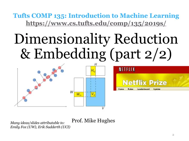
Tufts COMP 135: Introduction to Machine Learning https://www.cs.tufts.edu/comp/135/2019s/ Dimensionality Reduction & Embedding (part 2/2) Prof. Mike Hughes Many ideas/slides attributable to: Emily Fox (UW), Erik Sudderth (UCI) 2

What will we learn? Supervised Learning Data Examples Performance { x n } N measure Task n =1 Unsupervised Learning summary data of x x Reinforcement Learning Mike Hughes - Tufts COMP 135 - Spring 2019 3

Task: Embedding Supervised Learning x 2 Unsupervised Learning embedding Reinforcement x 1 Learning Mike Hughes - Tufts COMP 135 - Spring 2019 4

Dim. Reduction/Embedding Unit Objectives • Goals of dimensionality reduction • Reduce feature vector size (keep signal, discard noise) • “Interpret” features: visualize/explore/understand • Common approaches • Principal Component Analysis (PCA) + Factor Analysis • t-SNE (“tee-snee”) • word2vec and other neural embeddings • Evaluation Metrics • Storage size - Reconstruction error • “Interpretability” - Prediction error Mike Hughes - Tufts COMP 135 - Spring 2019 5

Example: Genes vs. geography Nature, 2008 Mike Hughes - Tufts COMP 135 - Spring 2019 6

Example: Genes vs. geography Nature, 2008 Where possible, we based the geographic origin on the observed country data for grandparents. We used a ‘strict consensus’ approach: if all observed grandparents originated from a single country, we used that country as the origin. If an individual’s observed grandparents originated from different countries, we excluded the individual. Where grandparental data were unavailable, we used the individual’s country of birth. Total sample size after exclusion: 1,387 subjects Features: over half a million variable DNA sites in the human genome Mike Hughes - Tufts COMP 135 - Spring 2019 7

Eigenvectors and Eigenvalues Mike Hughes - Tufts COMP 135 - Spring 2019 8

Source: https://textbooks.math.gatech.edu/ila/eigenvectors.html Mike Hughes - Tufts COMP 135 - Spring 2019 9

Demo: What is an Eigenvector? • http://setosa.io/ev/eigenvectors-and- eigenvalues/ Mike Hughes - Tufts COMP 135 - Spring 2019 10

Centering the Data Goal: each feature’s mean = 0.0 Mike Hughes - Tufts COMP 135 - Spring 2019 11

Why center? • Think of mean vector as simplest possible “reconstruction” of a dataset • No example specific parameters, just one F- dim vector N ( x n − m ) T ( x n − m ) X min m ∈ R F n =1 m ∗ = mean( x 1 , . . . x N ) Mike Hughes - Tufts COMP 135 - Spring 2019 12

Principal Component Analysis Mike Hughes - Tufts COMP 135 - Spring 2019 13

Reconstruction with PCA x i = Wz i + m + F vector K vector F x K F vector High- Low-dim Basis mean dim. vector data Mike Hughes - Tufts COMP 135 - Spring 2019 14

Principal Component Analysis Training step: .fit() • Input: • X : training data, N x F • N high-dim. example vectors • K : int, number of components • Satisfies 1 <= K <= F • Output: • m : mean vector, size F • W : learned basis of eigenvectors, F x K • One F-dim. vector (magnitude 1) for each component • Each of the K vectors is orthogonal to every other Mike Hughes - Tufts COMP 135 - Spring 2019 15

Principal Component Analysis Transformation step: .transform() • Input: • X : training data, N x F • N high-dim. example vectors • Trained PCA “model” • m : mean vector, size F • W : learned basis of eigenvectors, F x K • One F-dim. vector (magnitude 1) for each component • Each of the K vectors is orthogonal to every other • Output: • Z : projected data, N x K Mike Hughes - Tufts COMP 135 - Spring 2019 16

PCA Demo • http://setosa.io/ev/principal- component-analysis/ Mike Hughes - Tufts COMP 135 - Spring 2019 17

Example: EigenFaces Credit: Erik Sudderth Mike Hughes - Tufts COMP 135 - Spring 2019 18

PCA Principles • Minimize reconstruction error • Should be able to recreate x from z • Equivalent to maximizing variance • Want reconstructions to retain maximum information Mike Hughes - Tufts COMP 135 - Spring 2019 19

PCA: How to Select K? • 1) Use downstream supervised task metric • Regression error • 2) Use memory constraints of task • Can’t store more than 50 dims for 1M examples? Take K=50 • 3) Plot cumulative “variance explained” • Take K that seems to capture most or all variance Mike Hughes - Tufts COMP 135 - Spring 2019 20

Empirical Variance of Data X N F Var( X ) = 1 X X x 2 nf N n =1 f =1 N = 1 X x T n x n N n =1 • (Assumes each feature is centered) Mike Hughes - Tufts COMP 135 - Spring 2019 21

Variance of reconstructions N = 1 X x T n x n N n =1 N = 1 ( z n 1 w 1 + . . . + z nK w K ) T ( z n 1 w 1 + . . . + z nK w K ) X N n =1 N K = 1 X X z 2 nk N n =1 k =1 K Just sum up the top K eigenvalues! X λ k = k =1 Mike Hughes - Tufts COMP 135 - Spring 2019 22

Proportion of Variance Explained by first K components P K k =1 λ k PVE( K ) = P F f =1 λ f Mike Hughes - Tufts COMP 135 - Spring 2019 23

Variance explained curve Mike Hughes - Tufts COMP 135 - Spring 2019 24

PCA Summary PRO • Usually, fast to train, fast to test • Slowest step: finding K eigenvectors of an F x F matrix • Nested model • PCA with K=5 overlaps with PCA with K=4 CON • Sensitive to rescaling of input data features • Learned basis known only up to +/- scaling • Not often best for supervised tasks Mike Hughes - Tufts COMP 135 - Spring 2019 25

PCA: Best Practices • If features all have different units • Try rescaling to all be within (-1, +1) or have variance 1 • If features have same units, may not need to do this Mike Hughes - Tufts COMP 135 - Spring 2019 26

Beyond PCA: Factor Analysis Mike Hughes - Tufts COMP 135 - Spring 2019 27

A Probabilistic Model x i = Wz i + m + ✏ i F vector K vector F x K F vector F vector High- Low-dim Basis mean noise dim. vector data ✏ i ∼ N (0 , I F ) Mike Hughes - Tufts COMP 135 - Spring 2019 28

A Probabilistic Model x i = Wz i + m + ✏ i In terms of matrix math: X = WZ + M + E Mike Hughes - Tufts COMP 135 - Spring 2019 29

A Probabilistic Model x i = Wz i + m + ✏ i F vector K vector F x K F vector F vector High- Low-dim Basis mean noise dim. vector data   � 2 0 0 � 2 ✏ i ∼ N (0 , 0 0  )  � 2 0 0 Mike Hughes - Tufts COMP 135 - Spring 2019 30

Face Dataset  � 2  0 0 Is this noise model � 2 ✏ i ∼ N (0 , 0 0  ) realistic?  � 2 0 0 Mike Hughes - Tufts COMP 135 - Spring 2019 31

Each pixel might need own variance!  � 2  0 0 1 � 2 ✏ i ∼ N (0 , 0 0  )  2 � 2 0 0 3 Mike Hughes - Tufts COMP 135 - Spring 2019 32

Factor Analysis • Finds a linear basis like PCA, but allows per- feature estimation of variance  � 2  0 0 1 � 2 ✏ i ∼ N (0 , 0 0  )  2 � 2 0 0 3 • Small detail: columns of estimated basis may not be orthogonal Mike Hughes - Tufts COMP 135 - Spring 2019 33

PCA vs Factor Analysis Mike Hughes - Tufts COMP 135 - Spring 2019 34

Matrix Factorization and Singular Value Decomposition Mike Hughes - Tufts COMP 135 - Spring 2019 35

Matrix Factorization (MF) • User ! represented by vector " # ∈ % & ) ∈ % & • Item ' represented by vector ( * + ) approximates the utility , #) • Inner product " # • Intuition: • Two items with similar vectors get similar utility scores from the same user; • Two users with similar vectors give similar utility scores to the same item Mike Hughes - Tufts COMP 135 - Spring 2019 36

Mike Hughes - Tufts COMP 135 - Spring 2019 37

General Matrix Factorization X = ZW = Mike Hughes - Tufts COMP 135 - Spring 2019 38

SVD: Singular Value Decomposition Credit: Wikipedia Mike Hughes - Tufts COMP 135 - Spring 2019 39

Truncated SVD X = UDV T K K K K = Mike Hughes - Tufts COMP 135 - Spring 2019 40

Recall: Eigen Decomposition λ 1 , λ 2 , . . . λ K w 1 , w 2 , . . . w K Mike Hughes - Tufts COMP 135 - Spring 2019 41

Two ways to “fit” PCA • First, apply “centering” to X • Then, do one of these two options: • 1) Compute SVD of X • Eigenvalues are rescaled entries of the diagonal D • Basis = first K columns of V • 2) Compute covariance Cov(X) • Eigenvalues = largest eigenvalues of Cov(X) • Basis = corresponding eigenvectors of Cov(X) Mike Hughes - Tufts COMP 135 - Spring 2019 42

Visualization with t-SNE Mike Hughes - Tufts COMP 135 - Spring 2019 43

Reducing Dimensionality of Digit Images INPUT: Each image represented by 784-dimensional vector Apply PCA transformation with K=2 OUTPUT: Each image is a 2-dimensional vector Mike Hughes - Tufts COMP 135 - Spring 2019 44

Credit: Luuk Derksen (https://medium.com/@luckylwk/visualising-high-dimensional-datasets-using-pca-and-t-sne-in-python- 8ef87e7915b) Mike Hughes - Tufts COMP 135 - Spring 2019 45

Credit: Luuk Derksen (https://medium.com/@luckylwk/visualising-high-dimensional-datasets-using-pca-and-t-sne-in-python- 8ef87e7915b) Mike Hughes - Tufts COMP 135 - Spring 2019 46

Mike Hughes - Tufts COMP 135 - Spring 2019 47