Dijkstras Algorithm and the Bellman-Ford Algorithm Tyler Moore CSE - PDF document

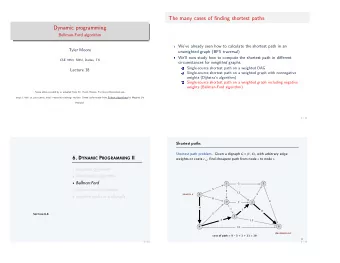
Notes Dijkstra’s Algorithm and the Bellman-Ford Algorithm Tyler Moore CSE 3353, SMU, Dallas, TX April 23, 2013 The many cases of finding shortest paths Notes We’ve already seen how to calculate the shortest path in an unweighted graph (BFS traversal) We’ll now study how to compute the shortest path in different circumstances for weighted graphs Single-source shortest path on a weighted DAG (review from last week) 1 Single-source shortest path on a weighted graph with nonnegative 2 weights (Dijkstra’s algorithm) Single-source shortest path on a weighted graph including negative 3 weights (Bellman-Ford algorithm) All-pairs shortest path on a weighted graph with nonnegative weights 4 Floyd-Warshall algorithm) 2 / 15 Shortest paths in DAGs Notes Key idea to dynamic programming: approach solutions as a sequential decision problem Each decision leads to new choices, and DP finds the best sequence of choices available Like greedy algorithms but less myopic Recursive approach to finding the shortest path from a to z Assume we already know the distance d ( v ) to z for each of a ’s 1 neighbors v ∈ G [ a ] Select the neighbor v that minimizes d ( v ) + W ( a , v ) 2 3 / 15 Recursive solution to finding shortest path in DAGs Notes r e c d a g s p (W, s , t ) : #Shortest path from s to t def @memo #Memoize f def d(u ) : #Distance from u to t u == t : return 0 # We ’ re there ! i f # Return the best of every f i r s t step return min (W[ u ] [ v]+d( v ) v in W[ u ] ) for return d( s ) #Apply f to a c t u a l s t a r t node 4 / 15

Shortest paths in DAGs: Iterative approach Notes The iterative solution is a bit more complicated We must start with a topological sort 1 Keep track of an upper bound on the distance from a to each node, 2 initialized to ∞ Go through each vertex and relax the distance estimate by inspecting 3 the path from the vertex to its neighbor In general, relaxing an edge ( u , v ) consists of testing whether we can shorten the path to v found so far by going through u ; if we can, we update d [ v ] with the new value Running time: Θ( m + n ) 5 / 15 Relaxing edges Notes s 1: d[v] = 13 2 : d [ u ] v = 2: W[u][v] = 3 7 u 6 / 15 Relaxing edges Notes s 3: d[v] = 13 10 2 : d [ u ] v = 2: W[u][v] = 3 7 u i n f = f l o a t ( ’ i n f ’ ) def r e l a x (W, u , v , D, P ) : d = D. get (u , i n f ) + W[ u ] [ v ] # P o s s i b l e s h o r t c u t estimate i f d < D. get ( v , i n f ) : # I s i t r e a l l y a s h o r t c u t ? D[ v ] , P[ v ] = d , u # Update estimate and parent True # There was a change ! return 6 / 15 Iterative solution to finding shortest path in DAGs Notes def dag sp (W, s , t ) : #Shortest path from s to t d = { u : f l o a t ( ’ i n f ’ ) for u in W } # Distance e s t i m a t e s d [ s ] = 0 #S t a r t node : Zero d i s t a n c e for u in t o p s o r t (W) : #In top − s o r t e d order . . . u == t : #Have we a r r i v e d ? i f break for v in W[ u ] : #For each out − edge . . . d [ v ] = min (d [ v ] , d [ u ] + W[ u ] [ v ] ) # Relax the edge return d [ t ] #Distance to t ( from s ) 7 / 15

But what if there are cycles? Notes With a DAG, we can select the order in which to visit nodes based on the topological sort With cycles we can’t easily determine the best order If there are no negative edges, we can traverse from the starting vertex, visiting nodes in order of their estimated distance from the starting vertex In Dijkstra’s algorithm, we use a priority queue based on minimum estimated distance from the source to select which vertices to visit Running time: Θ(( m + n ) lg n ) Dijkstra’s algorithm combines approaches seen in other algorithms Node discovery: bit like breadth-first traversal 1 Node visitation: selected using priority queue like Prim’s algorithm 2 Shortest path calculation: uses relaxation as in algorithm for shortest 3 paths in DAGs 8 / 15 Dijkstra’s algorithm Notes from heapq import heappush , heappop d i j k s t r a (G, s ) : def D, P, Q, S = { s :0 } , {} , [ ( 0 , s ) ] , s e t () # Est . , tree , queue , v i s i t e d while Q: # S t i l l unprocessed nodes ? , u = heappop (Q) # Node with lowest estimate i f u in S : continue # Already v i s i t e d ? Skip i t S . add (u) # We ’ ve v i s i t e d i t now for v in G[ u ] : # Go through a l l i t s neighbors r e l a x (G, u , v , D, P) # Relax the out − edge heappush (Q, (D[ v ] , v )) # Add to queue , w/ e s t . as p r i return D, P # F i n a l D and P returned 9 / 15 Dijkstra’s algorithm example Notes 1 b d 0 9 1 3 2 6 4 5 2 a c e 7 d[Node] : upper bd. dist. from a Node init. 1 (u=a) 2 (u=c) 3 (u=e) 4 (u=b) 5 (u=d) a 0 0 0 0 0 0 b ∞ 10 8 8 8 8 c ∞ 5 5 5 5 5 d ∞ ∞ 14 13 9 9 e ∞ ∞ 7 7 7 7 10 / 15 But what if there are negative edges? Notes With negative edges, we can’t select the next vertex to visit cleverly Instead, we just relax all m edges n times in a row If, after n rounds, the upper bounds don’t shrink, then we’ve found the shortest path from the source But if the upper bounds still shrink after n rounds, then there is a negative cycle in the graph, which is a problem (why?) Running time: Θ( m · n ) 11 / 15

Bellman-Ford Algorithm Notes def b el l ma n f or d (G, s ) : D, P = { s :0 } , {} # Zero − d i s t to s ; no parents rnd in G: # n = l e n (G) rounds for changed = False # No changes in round so f a r for u in G: # For every from − node . . . v in G[ u ] : # . . . and i t s to − nodes . . . for i f r e l a x (G, u , v , D, P ) : # Shortcut to v from u? changed = True # Yes ! So something changed i f not changed : break # No change in round : Done else : # Not done be f or e round n? ValueError ( ’ n e ga t i v e c y c l e ’ ) # Negative c y c l e detected r a i s e return D, P # Otherwise : D and P c o r r e c t 12 / 15 Bellman-Ford algorithm example Notes 5 x t Edge − 2 − Eval. 4 8 3 6 − Order 7 (t,x) (t,y) 7 9 y s z (t,z) (x,t) 2 (y,x) d[Node] : upper bd. dist. from s (y,z) Node init. 1 2 3 4 (z,x) s 0 0 0 0 0 (z,s) (s,t) t ∞ 6 6 2 2 x ∞ ∞ 114 4 4 (s,y) y ∞ 7 7 7 7 z ∞ ∞ 2 2 -2 13 / 15 From single-source to all-pairs shortest paths Notes The algorithms discussed so far calculated the shortest path to all vertices from a single source We might instead be interested in the shortest path to all vertices from all sources We could run Dijkstra’s or Bellman-Ford n times, one for each source But more efficient solutions exist, particularly when graphs are dense 14 / 15 All-pairs shortest path application Notes Let’s compare distances between airport hubs City New York Los Angeles Seattle Atlanta Dallas New York 0 2470 2400 760 1390 LA 2470 0 1940 1230 Seattle 2400 1908 0 2180 1660 Atlanta 760 1940 2180 0 729 Dallas 1390 1230 1660 729 0 Total 7020 7548 8148 5609 5009 The farness of a node in a connected graph is the sum of all shortest path distances to other nodes Closeness centrality: inverse of the average length of all shortest paths from a vertex 15 / 15