Digital Audio Effects Graduate School of Culture Technology, KAIST - PowerPoint PPT Presentation
2018 Fall CTP431: Music and Audio Computing Digital Audio Effects Graduate School of Culture Technology, KAIST Juhan Nam Introduction Amplitude - Gain, fade in/out, automation curve, compressor Timbre - Filters, EQ, distortion,
2018 Fall CTP431: Music and Audio Computing Digital Audio Effects Graduate School of Culture Technology, KAIST Juhan Nam
Introduction • Amplitude - Gain, fade in/out, automation curve, compressor • Timbre - Filters, EQ, distortion, modulation, flanger, vocoder • Pitch - Pitch shifting, transpose • Time stretching - Timing change, tempo adjustment • Spatial effect - Delay, Reverberation, panning, binaural (HRTF) Source: http://www.uaudio.com/uad/downloads Source: https://www.izotope.com/en/products/repair-and-edit/rx-post-production-suite.html
Let’s first enjoy some effects! • http://webaudioplayground.appspot.com
Digital System Digital Input Output System ! " # " • Take the input signal ! " as a sequence of numbers and returns the output signal # " as another sequence of numbers • We are particularly interested in linear systems that are composed of the following operations - Multiplication: # " = % & ' ! " - Delaying: # " = ! " − 1 - Summation: # " = ! " + ! " − 1
Linear Time-Invariant (LTI) System Digital Input Output System ! " $ " • Linearity - Homogeneity: if ! " → $ " , then a & ! " → a & $ " - Superposition: if ! ' " → $ ' " and ! ( " → $ ( (n) , then ! ' " + ! ( " → $ ' " + $ ( " • Time-Invariance - If ! " → $ " , then ! " − + → $ " − + for any + - This means that the system does not change its behavior over time
LTI System • LTI systems in frequency domain - No new sinusoidal components are introduced - Only existing sinusoids components changes in amplitude and phase. • Examples of non-LTI systems - Clipping - Distortion - Aliasing - Modulation
LTI Digital Filters • A LTI digital filters performs a combination of the three operations - " # = % & ' ( # + % * ' ( # − 1 + % - ' ( # − 2 + ⋯ + % 0 ' ( # − 1 • This is a general form of Finite Impulse Response (FIR) filter
Two Ways of Defining LTI Systems • By the relation between input ! " and output # " - Difference equation - Signal flow graph • By the impulse response of the system - Measure it by using a unit impulse as input - Convolution operation
The Simplest Lowpass Filter • Difference equation ! " = $ " + $(" − 1) • Signal flow graph + $ " ! " * +, “Delay Operator”
The Simplest Lowpass Filter: Sine-Wave Analysis • Measure the amplitude and phase changes given a sinusoidal signal input
The Simplest Lowpass Filter: Frequency Response • Plot the amplitude and phase change over different frequency - The frequency sweeps from 0 to the Nyquist rate
The Simplest Lowpass Filter: Frequency Response • Mathematical approach - Use complex sinusoid as input: ! " = $ %&' - Then, the output is: ( " = ! " + ! " − 1 = $ %&' + $ %&('-.) = 1 + $ -%& 0 $ %&' = 1 + $ -%& 0 !(") - Frequency response: 1 2 = 1 + $ -%& = $ % 3 4 + $ -% 3 4 $ -% 3 9 )$ -% 3 & 4 = 2cos( 4 & - Amplitude response: 1(2) = 2 cos 9 & - Phase response: ∠1 2 = − 9
The Simplest Highpass Filter • Difference equation: ! " = $ " − $(" − 1) • Frequency response
Impulse Response Output Input Filter + # = ℎ(#) " # = % # ℎ # • The filter output when the input is a unit impulse - " # = % # = 1, 0, 0, 0, … → + # = ℎ(#) • Characterizes the digital system as a sequence of numbers - A system is represented just like audio samples!
Examples: Impulse Response • The simplest lowpass filter - h ! = 1, 1 • The simplest highpass filter - h ! = 1, −1 • Moving-average filter (order=5) & & & & & - h ! = ' , ' , ' , ' , ' • General FIR Filter - h ! = ( ) , ( & , ( * , … , ( , à A finite length of impulse response
Convolution • The output of LTI digital filters is represented by convolution operation between ! " and ℎ " * 3 " = ! " ∗ ℎ " = ; !(8) + ℎ(" − 8) 56% • Deriving convolution - The input can be represented as a time-ordered set of weighted impulses � ! " = ! % , ! ' , ! ( , … , ! * = ! % + , " + ! ' + , " − 1 + ! ( + , " − 2 + ⋯ + ! * + , " − 2 - By the linearity and time-invariance � 3 " = ! % + ℎ " + ! ' + ℎ " − 1 + ! ( + ℎ " − 2 + ⋯ + ! * + ℎ " − 2 = * !(8) + ℎ(" − 8) ∑ 56%
Convolution In Practice • The practical expression of convolution + + $ " = ! " ∗ ℎ " = ' ! , - ℎ " − , = ' ℎ(,) - !(" − ,) ()* ()* - This represents input ! " as a streaming data to the filter ℎ " • The length of convolution output - If the length of ! " is M and the length of ℎ " is N , the length of $ " is M+N-1
Demo: Convolution
Feedback Filter + Output Input Filter ! " . " Delay • LTI digital filters allow to use the past outputs as input - Past outputs: ! " − 1 , ! " − 2 , … , ! " − ( • The whole system can be represented as - ! " = + , - . " + 0 1 - ! " − 1 + 0 2 - ! " − 2 + ⋯ + 0 4 - ! " − ( - This is a general form of Infinite Impulse Response (IIR) filter
A Simple Feedback Lowpass Filter • Difference equation " # = % # + ! ' "(# − 1) • Signal flow graph + % # " # , -. ! - When ! is slightly less than 1, it is called “Leaky Integrator”
A Simple Feedback Lowpass Filter: Impulse Response • Impulse response - " 0 = % 0 = 1 - " 1 = % 1 + ( ) " 0 = ( - " 2 = % 2 + ( ) " 1 = ( + - … - " , = % , + ( ) " , − 1 = ( . • Stability! - If ( < 1 , the filter output converges (stable) - If ( = 1 , the filter output oscillates (critical) - If ( > 1 , the filter output diverges (unstable)
A Simple Feedback Lowpass Filter: Frequency Response • More dramatic change than the simplest lowpass filter (FIR) - Phase response is not linear ! " = $ " + 0.9 ) !(" − 1)
Reson Filter • Difference equation ! " = $ " + 2' ( cos, ( ! " − 1 − ' / ( ! " − 2 • Signal flow graph + ! " $ " + 0 12 2' ( cos, + 0 12 −' /
Reson Filter: Frequency Response • Generate resonance at a particular frequency - Control the peak height by ! and the peak frequency by " For stability: ! < 1
Bi-quad Filter • Difference equation $ % = ' ( ) * % + ' # ) * % − 1 + ' . ) * % − 2 − 0 # ) $ % − 1 − 0 . ) $ % − 2 • Signal flow graph y(n) + x(n) b 0 ! "# ! "# x(n-1) y(n-1) b 1 -a 1 ! "# ! "# x(n-2) y(n-2) b 2 -a 2
Frequency Response • Sine-wave Analysis - " # = % &'( à " # − * = % &'((,-) = % ,&'- " # for any * - Let’s assume that / # = 0 1 % &('(23 ' ) à / # − * = % ,&'- / # for any * • Putting this into the different equation / # = 4 5 8 " # + 4 7 8 % ,&' 8 " # + 4 9 8 % ,&9' 8 " # − ; 7 8 % ,&' 8 / # − ; 9 8 % ,&9' 8 / # / # = 4 5 + 4 7 8 % ,&' + 4 9 8 % ,&9' 1 + ; 7 8 % ,&' + ; 9 8 % ,&9' "(#) <(1) : frequency response <(1) = 4 5 + 4 7 8 % ,&' + 4 9 8 % ,&9' 0 1 = <(1) : amplitude response 1 + ; 7 8 % ,&' + ; 9 8 % ,&9' = 1 = ∠<(1) : phase response
Z-Transform • ! -transform - Define z to be a variable in complex plane: we call it z -plane - When z = e j ω (on unit circle), the frequency response is a particular case of the following form *(") = + , + + $ . " #$ + + / . " #/ % " = '(") 1 + 1 $ . " #$ + 1 / . " #/ - We call this " -transform or the transfer function of the filter - z -1 corresponds to one sample delay: delay operator or delay element - Filters are often expressed as " -transform: polynomial of " #$
Practical Filters • One-pole one-zero filters - Leaky integrator 1 z − 1 H ( z ) = b 0 + b - Moving average a 0 + a 1 z − 1 - DC-removal filters - Bass / treble shelving filter • Biquad filters 1 z − 1 + b 2 z − 2 H ( z ) = b 0 + b - Reson filter a 0 + a 1 z − 1 + a 2 z − 2 - Band-pass / notch filters - Equalizer • Any high-order filter can be factored into a combination of one- pole one-zero filters or bi-quad filters!
Low-pass Filter • Transfer Function 1 + 2 z − 1 + 1 z − 2 α = sin Θ H ( z ) = (1 − cos Θ ) Θ = 2 π f c / f s (1 + α ) − 2cos Θ z − 1 + (1 − α ) z − 2 2 Q 2 - fc : cut-off frequency, Q: resonance Lowpass Filters Lowpass Filters 30 30 20 20 Q =4 10 10 Q =2 Gain(dB) Gain(dB) Q =1 f=400 f=1000 f=3000 f=8000 0 0 Q =0.5 − 10 − 10 − 20 − 20 − 30 − 30 2 3 4 2 3 4 10 10 10 10 10 10 freqeuncy(log10) freqeuncy(log10)
High-pass Filter • Transfer Function 1 − 2 z − 1 + 1 z − 2 H ( z ) = (1 + cos Θ α = sin Θ ) Θ = 2 π f c / f s (1 + α ) − 2cos Θ z − 1 + (1 − α ) z − 2 2 2 Q Highpass Filters Highpass Filters 30 30 20 20 f=400 f=1000 f=3000 f=8000 Q =4 10 10 Q =2 Gain(dB) Gain(dB) Q =1 0 0 Q =0.5 − 10 − 10 − 20 − 20 − 30 − 30 2 3 4 2 3 4 10 10 10 10 10 10 freqeuncy(log10) freqeuncy(log10)
Recommend
More recommend
Explore More Topics
Stay informed with curated content and fresh updates.

