Diffusion Models in Population Genetics Laura Kubatko - PowerPoint PPT Presentation
Diffusion Models in Population Genetics Laura Kubatko kubatko.2@osu.edu MBI Workshop on Spatially-varying stochastic differential equations, with application to the biological sciences July 10, 2015 Laura Kubatko Diffusion Models in
Diffusion Models in Population Genetics Laura Kubatko kubatko.2@osu.edu MBI Workshop on Spatially-varying stochastic differential equations, with application to the biological sciences July 10, 2015 Laura Kubatko Diffusion Models in Population Genetics July 10, 2015 1 / 24
Population Genetics Population genetics: Study of genetic variation within a population Assume that a gene has two alleles, call them A and a Population is composed of N individuals who have two copies of each gene – so possible genotypes are: AA Aa aa The population evolves over time We are interested in the composition of the population at generation t Need a model for how a generation is derived from the previous generation Laura Kubatko Diffusion Models in Population Genetics July 10, 2015 2 / 24
Wright-Fisher Model Assumptions: ◮ Population of 2 N gene copies ◮ Discrete, non-overlapping generations of equal size ◮ Parents of next generation of 2 N genes are picked randomly with replacement from preceding generation (genetic differences have no fitness consequences) ◮ Probability of a specific parent for a gene in the next generation is 1 2 N Laura Kubatko Diffusion Models in Population Genetics July 10, 2015 3 / 24
Wright-Fisher Model Source: Popvizard, a python program to simulate evolution under the WF and other models, written by Peter Beerli http://people.sc.fsu.edu/ pbeerli/popvizard.tar.gz Laura Kubatko Diffusion Models in Population Genetics July 10, 2015 4 / 24
The Wright-Fisher Model View Wright-Fisher model as a discrete-time Markov process Let Y t = number of alleles of type A in population at generation t , 0 ≤ Y t ≤ 2 N for t = 0 , 1 , . . . Define p ij = P ( Y t +1 = j | Y t = i ). Then, �� 2 N ( i 2 N ) j ( 2 N − i 2 N ) 2 N − j , � j = 0 , 1 , . . . , 2 N j p ij = 0 , otherwise States 0 and 2 N are absorbing states – we can never leave these states Laura Kubatko Diffusion Models in Population Genetics July 10, 2015 5 / 24
The Wright-Fisher Model Note that: ◮ E ( Y t +1 | Y t = i ) = 2 N ( i 2 N ) = i ◮ Var ( Y t +1 | Y t = i ) = 2 N ( i i 2 N )(1 − 2 N ) ◮ So the expected number of A alleles remains the same, but the actual number may vary between 0 and 2 N Classical approach: Look at the limit as the population size N → ∞ Kingman’s Coalescent Process ◮ Widely used in population genetics and phylogenetics ◮ Difficult to extend to handle features of the evolutionary process, such as selection Laura Kubatko Diffusion Models in Population Genetics July 10, 2015 6 / 24
Wright-Fisher Model as a Diffusion Process Define a diffusion process { X t } t ≥ 0 as a continuous-time Markov process with approximately Guassian increments over small time intervals and for which the following three conditions hold for small δ t and X t = x : ◮ E ( X t + δ t − X t | X t = x ) = µ ( t , x ) δ t + o ( δ t ) ◮ E (( X t + δ t − X t ) 2 | X t = x ) = σ 2 ( t , x ) δ t + o ( δ t ) ◮ E (( X t + δ t − X t ) k | X t = x ) = 0 for k > 2 From Radu’s slides, we had: dX t = S ( X t ) dt + σ ( X t ) dW t , where S ( X t ) is the drift coefficient and σ ( X t ) is the diffusion coefficient. For standard Brownian Motion, µ ( t , x ) = 0 and σ 2 ( t , x ) = 1. Laura Kubatko Diffusion Models in Population Genetics July 10, 2015 7 / 24
Wright-Fisher Model as a Diffusion Process Let Y t be the number of A alleles in the population at generation t Let X t = proportion of A alleles in population at generation t ; X t = Y t 2 N Let X t represent the continuous-time process (eventually measure time in units of 2 N generations, as before) Define ∆ Y t = Y t +1 − Y t and ∆ X t = X t +1 − X t Then E ( Y t +1 | X t = x ) = 2 Nx E (∆ Y t | X t = x ) = 0 E [(∆ Y t ) 2 | X t = x )] = 2 Nx (1 − x ) E (∆ X t | X t = x ) = 0 = µ ( t , x ) = µ ( x ) E ((∆ X t ) 2 | X t = x ) = x (1 − x ) = σ 2 ( t , x ) = σ 2 ( x ) 2 N Laura Kubatko Diffusion Models in Population Genetics July 10, 2015 8 / 24
Wright-Fisher Model as a Diffusion Process Now re-define ∆ Y t = Y t +∆ t − Y t and ∆ X t = X t +∆ t − X t , 2 N and let N → ∞ , so that E ((∆ X t ) 2 | X t ) = X t (1 − X t )∆ t 1 where ∆ t = The corresponding SDE is � d X t = X t (1 − X t ) d W t , X t ∈ [0 , 1] where W t is standard Brownian Motion (See Pardoux, 2009, for a rigorous proof) Laura Kubatko Diffusion Models in Population Genetics July 10, 2015 9 / 24
The Wright-Fisher Model with Selection Model for selection: ◮ Suppose that allele A is superior to allele a so that 2 Nx (1 + s ) p x = 2 Nx (1 + s ) + (2 N − 2 Nx ) ◮ As before, let N → ∞ and define s = β/ (2 N ). ◮ E (∆ X t | X t ) ≈ ( β X t (1 − X t ))∆ t ◮ E ((∆ X t ) 2 | X t ) ≈ X t (1 − X t )∆ t The corresponding SDE is � d X t = β X t (1 − X t ) dt + X t (1 − X t ) d W t , X t ∈ [0 , 1] Laura Kubatko Diffusion Models in Population Genetics July 10, 2015 10 / 24
The Wright-Fisher Diffusion with Selection: Intuition Use the Euler Method (see Radu’s lectures) to simulate from the WF Diffusion model X ( t i +1 ) = X ( t i ) + β X ( t i )(1 − X ( t i ))( t i +1 − t i ) + √ t i +1 − t i � X ( t i )(1 − X ( t i )) Z where Z ∼ N (0 , 1) Python code to simulate this: ◮ T = 0 . 05 ◮ Define 0 = t 0 < t 1 < · · · < t N − 1 < t N = T , equally spaced ◮ Vary β Laura Kubatko Diffusion Models in Population Genetics July 10, 2015 11 / 24
The Wright-Fisher Diffusion with Selection: Intuition β = 0, varying N Laura Kubatko Diffusion Models in Population Genetics July 10, 2015 12 / 24
The Wright-Fisher Diffusion with Selection: Intuition N = 1000, vary β Laura Kubatko Diffusion Models in Population Genetics July 10, 2015 13 / 24
Application: Inferring Selection From Genome-scale Data Diffusion models are currently becoming more widely used in analyzing genome-scale data. Example: Williamson, S. H. et al. 2005. Simultaneous inference of selection and population growth from patterns of variation in the human genome. PNAS: 120(22): 7882-7887. Data: NIEHS Environmental Genome Project web site (http://egp.gs.washington. edu) ◮ Sequenced 301 genes associated with variation in response to environmental exposure ◮ 90 individuals: 24 African Americans, 24 Asian Americans, 24 European Americans, 12 Mexican Americans, and 6 Native Americans Goal: Detect selection in different types of mutations; distinguish selection from other demographic factors, such as population size change Laura Kubatko Diffusion Models in Population Genetics July 10, 2015 14 / 24
Application: Inferring Selection From Genome-scale Data Data are recorded as SNPs – bases in the DNA sequence at which there is variation across individuals Example data: Taxon Sequence (A) Human GCCGATGCCGATGCCGAA (B) Chimp GCCGTTGCCGTTGCCGTT (C ) Gorilla GCGGAAGCGGAAGCGGAA this would be Taxon Sequence (A) Human CATCATCAA (B) Chimp CTTCTTCTT (C ) Gorilla GAAGAAGAA Laura Kubatko Diffusion Models in Population Genetics July 10, 2015 15 / 24
Application: Inferring Selection From Genome-scale Data Example SNP data is Taxon Sequence (A) Human CATCATCAA (B) Chimp CTTCTTCTT (C ) Gorilla GAAGAAGAA Record this as the site frequency spectrum (SFS), denoted by the vector u , where entry u i = number of SNP sites with i copies of the derived allele For the example, we have (assuming that the ancestral state is that found in Gorilla), u = (4 , 5) If we let Human be ancestral, we’d have u = (9 , 0) Laura Kubatko Diffusion Models in Population Genetics July 10, 2015 16 / 24
Application: Inferring Selection From Genome-scale Data Idea of analysis: ◮ Write the likelihood function and obtain MLEs of the parameters of interest ◮ Likelihood function for a sample of K SNPs: K � L ( β ) = Pr ( i k , n k | β ) k =1 i k where Pr ( i k , n k ) is the probability of that SNP k is at frequency n k Pr ( i k , n k ) comes from the diffusion model – how? ◮ Williamson et al. (2005): Use numerical methods to approximate the diffusion ◮ Today: use a naive sampling method based on the Euler approximation ◮ Ongoing work (with Radu Herbei and Jeff Gory): use exact sampling from the WF diffusion to implement a Bayesian version of the model Laura Kubatko Diffusion Models in Population Genetics July 10, 2015 17 / 24
Application: Inferring Selection From Genome-scale Data Naive method: Use the Euler method to simulate a path from the WF diffusion with selection 1 parameter β , and record the final allele frequency, q . For the q from step 1, simulate the data for a SNP by drawing 2 Y ∼ Bin (2 n , q ). n is the number of “people” in the sample. Repeat steps 1-2 a large number of times, say M (the larger, the better), to 3 generate a set of observed Y values, Y 1 , Y 2 , · · · , Y M . Form the estimates ˆ 1 � M P i ( β ) = m =1 I ( Y m = i ) 4 M The approximate likelihood is then K ˆ � ˆ L ( β ) = P i k ( β ) k =1 Laura Kubatko Diffusion Models in Population Genetics July 10, 2015 18 / 24
Application: Inferring Selection From Genome-scale Data Does it work? Simulate data for 15 people and 100 SNPs with various values of β and M β = 0 . 2 Laura Kubatko Diffusion Models in Population Genetics July 10, 2015 19 / 24
Application: Inferring Selection From Genome-scale Data Does it work? Simulate data for 15 people and 100 SNPs with various values of β and M β = 2 . 0 Laura Kubatko Diffusion Models in Population Genetics July 10, 2015 20 / 24
Recommend
More recommend
Explore More Topics
Stay informed with curated content and fresh updates.
