Dependence Properties of Reduced-form portfolio credit risk model - PowerPoint PPT Presentation

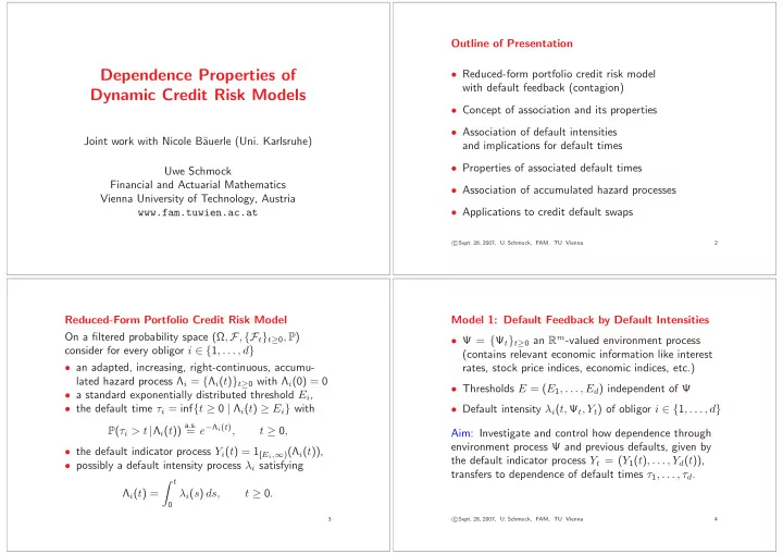
Outline of Presentation Dependence Properties of • Reduced-form portfolio credit risk model with default feedback (contagion) Dynamic Credit Risk Models • Concept of association and its properties • Association of default intensities Joint work with Nicole B¨ auerle (Uni. Karlsruhe) and implications for default times • Properties of associated default times Uwe Schmock Financial and Actuarial Mathematics • Association of accumulated hazard processes Vienna University of Technology, Austria • Applications to credit default swaps www.fam.tuwien.ac.at c � Sept. 28, 2007, U. Schmock, FAM, TU Vienna 2 Reduced-Form Portfolio Credit Risk Model Model 1: Default Feedback by Default Intensities On a filtered probability space (Ω , F , {F t } t ≥ 0 , P ) • Ψ = { Ψ t } t ≥ 0 an R m -valued environment process consider for every obligor i ∈ { 1 , . . . , d } (contains relevant economic information like interest • an adapted, increasing, right-continuous, accumu- rates, stock price indices, economic indices, etc.) lated hazard process Λ i = { Λ i ( t ) } t ≥ 0 with Λ i (0) = 0 • Thresholds E = ( E 1 , . . . , E d ) independent of Ψ • a standard exponentially distributed threshold E i , • the default time τ i = inf { t ≥ 0 | Λ i ( t ) ≥ E i } with • Default intensity λ i ( t, Ψ t , Y t ) of obligor i ∈ { 1 , . . . , d } a.s. = e − Λ i ( t ) , P ( τ i > t | Λ i ( t )) t ≥ 0 , Aim: Investigate and control how dependence through environment process Ψ and previous defaults, given by • the default indicator process Y i ( t ) = 1 [ E i , ∞ ) (Λ i ( t )), the default indicator process Y t = ( Y 1 ( t ) , . . . , Y d ( t )), • possibly a default intensity process λ i satisfying transfers to dependence of default times τ 1 , . . . , τ d . � t Λ i ( t ) = λ i ( s ) ds, t ≥ 0 . 0 c 3 � Sept. 28, 2007, U. Schmock, FAM, TU Vienna 4

Definition of Association Association is Notion for Positive Dependence Let ( X, Y ) be an R 2 -valued random vector with mar- • An R d -valued random vector X = ( X 1 , . . . , X d ) and ginal distributions F and G . its distribution L ( X ) are called associated, if Definition: Kendall’s τ Cov( f ( X ) , g ( X )) ≥ 0 τ K ( X, Y ) := E [sign( X − X ′ ) sign( Y − Y ′ )] , with ( X ′ , Y ′ ) an independent copy of ( X, Y ). for all measurable, componentwise increasing functions f, g : R d → R for which f ( X ), g ( X ) and Definition: Spearman’s ̺ the product f ( X ) g ( X ) are integrable. ̺ S ( X, Y ) := Corr[ F ( X ) G ( Y )] • An R d -valued process { X t } t ≥ 0 is called associated Lemma: ∗ If ( X, Y ) is associated, then τ K ( X, Y ) ≥ 0 if for all k ∈ N and times 0 ≤ t 1 < · · · < t k the and ̺ S ( X, Y ) ≥ 0. R dk -valued vector ( X ( t 1 ) , . . . , X ( t k )) is associated. ∗ cf. Nelsen, An Introduction to Copulas, Springer (1999) c 5 � Sept. 28, 2007, U. Schmock, FAM, TU Vienna 6 Properties of Association ∗ Association is a Copula Property Let X = ( X 1 , . . . , X d ) be an R d -valued random • If X 1 , . . . , X d are independent, then the random vector X = ( X 1 , . . . , X d ) is associated. vector with marginal distributions F 1 , . . . , F d . Define the copula C X : [0 , 1] d → [0 , 1] of X as distribution • If X = ( X 1 , . . . , X d ) and Y = ( Y 1 , . . . , Y k ) are function of ( F 1 ( X 1 ) , . . . , F d ( X d )). associated random vectors, which are independent, then ( X 1 , . . . , X d , Y 1 , . . . , Y k ) is associated. Lemma: X is associated ⇐ ⇒ C X is associated. • If X = ( X 1 , . . . , X d ) is associated, then the vector Proof: “= ⇒ ” By property of association. ( f 1 ( X ) , . . . , f k ( X )) is associated for every k ∈ N “ ⇐ =” Use the lower quantile functions and every choice of measurable increasing (or decreasing) functions f 1 , . . . , f k : R d → R . F ← i ( t ) := inf { x ∈ R | F i ( x ) ≥ t } , t ∈ [0 , 1] , • If { X n } n ∈ N is a sequence of associated R d -valued for i ∈ { 1 , . . . , d } to see that d random vectors and X n → X , then X is associated. a.s. F ← 1 ( F 1 ( X 1 )) , . . . , F ← ∗ see Esary, Proschan, Walkup (1967), Ann. Math. Statist. 38 � � ( X 1 , . . . , X d ) = d ( F d ( X d )) . c 7 � Sept. 28, 2007, U. Schmock, FAM, TU Vienna 8

Application to Defaultable Zero-Coupon Bonds Conditional Increasing in Sequence and Association Let R t denote the integrated stochastic interest inten- Definition: X = ( X 1 , . . . , X d ) is called conditional sity, i.e., e − R t is the factor for discounting from t to 0. increasing in sequence (CIS) if for every k ∈ { 2 , . . . , d } Let Λ t denote the accumulated hazard for default up to t . and bounded increasing f : R → R Lemma: For a defaultable payment of 1 at time t , ( x 1 , . . . , x k − 1 ) �→ E [ f ( X k ) | X 1 = x 1 , . . . , X k − 1 = x k − 1 ] assume that ( R t , Λ t ) is associated under an equivalent pricing measure P . Then for the price at time 0: is increasing in every x 1 , . . . , x k − 1 . E [ e − R t 1 { τ>t } ] ≥ E [ e − R t ] P ( τ > t ) . Lemma: ∗ If X is conditional increasing in sequence, then X is associated. Proof: The vector ( e − R t , e − Λ t ) is associated. Since { τ > t } = { Λ t < E } and P (Λ t < E | Λ t , R t ) = e − Λ t , Remark: CIS is convenient for Markov processes. the definition of association implies ∗ cf. A. M¨ uller & D. Stoyan, Comparison Methods for Stochastic e − R t 1 { τ>t } e − R t e − Λ t � e − R t � e − Λ t � � � � � � = E ≥ E E E . Models and Risks, Wiley (2002), Theorem 3.10.11. c 9 � Sept. 28, 2007, U. Schmock, FAM, TU Vienna 10 Examples of Associated (Environment) Processes Monotone Mixtures and Association • R d -valued process { X t } t ≥ 0 with independent, associ- Definition: X = ( X 1 , . . . , X d ) is called a monotone ated increments X t − X s , 0 ≤ s < t . This includes mixture of Θ = (Θ 1 , . . . , Θ k ) if for every measurable, bounded and componentwise increasing f : R d → R deterministic time changes of 1-dim. L´ evy processes. • Interest rate process { r t } t ≥ 0 in Vasicek’s model is there exists a measurable, componentwise increasing h : R k → R such that CIS because for all 0 ≤ s < t � t a.s. � � h (Θ) = E f ( X ) | Θ r t = m + ( r s − m ) e − κ ( t − s ) + σ . e − κ ( t − u ) dW u . s Lemma: ∗ If the conditional distribution L ( X | Θ) is • Birth-and-death processes are CIS. associated, Θ is associated and X is a monotone • Interest rate process { r t } t ≥ 0 in Cox-Ingersoll-Ross mixture of Θ, then the vector ( X, Θ) is associated. model is CIS. ∗ see K. Jogdeo (1978), Ann. Statist. 6, 232–234. • Volatility processes of GARCH(1,1) processes c 11 � Sept. 28, 2007, U. Schmock, FAM, TU Vienna 12

Implication of Associated (Integrated) Intensities Association in Model 1 with Default Intensities Theorem: (B. & S.) If � � for the joint R d -valued Write λ t = λ 1 ( t ) , . . . , λ d ( t ) � � intensity process and Λ t = Λ 1 ( t ) , . . . , Λ d ( t ) for the • environment process Ψ is associated, • λ i ( t, Ψ t , Y t ) is increasing in 2 nd and 3 rd argument, integrated version (accumulated hazard) at time t ≥ 0. � ∞ a.s. = ∞ for every y ∈ { 0 , 1 } d , y i = 0, • λ i ( t, Ψ t , y ) dt Lemma: (B. & S.) 0 • technical conditions (suitable meas. & continuity), • If { λ t } t ≥ 0 is associated and c` adl` ag, then { Λ t } t ≥ 0 is associated. then the accumulated hazard process �� t • If { Λ t } t ≥ 0 is associated, right-continuous and � Λ t = λ i ( s, Ψ s , Y s ) ds t ≥ 0 , , Λ i ( t ) ր ∞ a.s. as t → ∞ for every i ∈ { 1 , . . . , d } , 0 i =1 ,...,d and the thresholds ( E 1 , . . . , E d ) are associated and independent of { Λ t } t ≥ 0 , then the default times is associated, and the default times τ = ( τ 1 , . . . , τ d ) are ( τ 1 , . . . , τ d ) are associated. associated, too. c 13 � Sept. 28, 2007, U. Schmock, FAM, TU Vienna 14 Association and Positive Supermodular Dependence Implications of Associated Default Times Definition: f : R d → R is called supermodular if If ( τ 1 , . . . , τ d ) are associated, then, for all non-void I ⊂ { 1 , . . . , d } and { t i } i ∈ I ⊂ [0 , ∞ ), ∀ x, y ∈ R d . f ( x ) + f ( y ) ≤ f ( x ∨ y ) + f ( x ∧ y ) , P ( τ ⊥ Definition: Let X = ( X 1 , . . . , X d ) be a random vector i > t i for all i ∈ I ) ≤ P ( τ i > t i for all i ∈ I ) , and X ⊥ = ( X ⊥ 1 , . . . , X ⊥ d ) a copy with independent P ( τ ⊥ i ≤ t i for all i ∈ I ) ≤ P ( τ i ≤ t i for all i ∈ I ) , components. Then X and its distribution L ( X ) are called positive supermodular dependent (PSD) if because the indicator functions are supermodular. E [ f ( X ⊥ )] ≤ E [ f ( X )] Definition: A r.v. X is smaller in usual stochastic order for all measurable, supermodular f : R d → R for which than Y , if P ( X > t ) ≤ P ( Y > t ) for all t ∈ R . the expectations exist. Consequence: With ≤ st for usual stochastic order, Lemma: ∗ X is associated = ⇒ X is PSD. i ∈ I τ ⊥ i ∈ I τ ⊥ min i ≤ st min and max i ∈ I τ i ≤ st max i ∈ I τ i i . ∗ cf. Christofides, Vaggelatou (2004), J. Multivariate Anal. 88. c 15 � Sept. 28, 2007, U. Schmock, FAM, TU Vienna 16