DEPARTMENT OF MATHEMATICS AND STATISTICS Memorial University of - PDF document

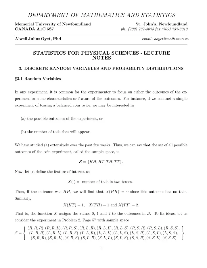
DEPARTMENT OF MATHEMATICS AND STATISTICS Memorial University of Newfoundland St. John’s, Newfoundland CANADA A1C 5S7 ph. (709) 737-8075 fax (709) 737-3010 Alwell Julius Oyet, Phd email: aoyet@math.mun.ca STATISTICS FOR PHYSICAL SCIENCES - LECTURE NOTES 3. DISCRETE RANDOM VARIABLES AND PROBABILITY DISTRIBUTIONS § 3.1 Random Variables In any experiment, it is common for the experimenter to focus on either the outcomes of the ex- periment or some characteristics or feature of the outcomes. For instance, if we conduct a simple experiment of tossing a balanced coin twice, we may be interested in (a) the possible outcomes of the experiment, or (b) the number of tails that will appear. We have studied (a) extensively over the past few weeks. Thus, we can say that the set of all possible outcomes of the coin experiment, called the sample space, is S = { HH, HT, TH, TT } . Now, let us de fi ne the feature of interest as X ( · ) = number of tails in two tosses. Then, if the outcome was HH , we will fi nd that X ( HH ) = 0 since this outcome has no tails. Similarly, X ( HT ) = 1 , X ( TH ) = 1 and X ( TT ) = 2 . That is, the function X assigns the values 0, 1 and 2 to the outcomes in S . To fi x ideas, let us consider the experiment in Problem 2, Page 57 with sample space    ( R, R, R ) , ( R, R, L ) , ( R, R, S ) , ( R, L, R ) , ( R, L, L ) , ( R, L, S ) , ( R, S, R ) , ( R, S, L ) , ( R, S, S ) ,    S = ( L, R, R ) , ( L, R, L ) , ( L, R, S ) , ( L, L, R ) , ( L, L, L ) , ( L, L, S ) , ( L, S, R ) , ( L, S, L ) , ( L, S, S ) ,  .    ( S, R, R ) , ( S, R, L ) , ( S, R, S ) , ( S, L, R ) , ( S, L, L ) , ( S, L, S ) , ( S, S, R ) , ( S, S, L ) , ( S, S, S ) 1

De fi ne the rule, X = number of cars that turned right. We fi nd that X ( R, R, R ) = 3 , X ( R, L, R ) = 2 , X ( R, S, L ) = 1 , X ( L, L, L ) = 0 , and so on. If we enumerate all the values that X assigns to the outcomes in S , we will fi nd that the possible values of X are 0, 1, 2, and 3. The value 0 will occur 8 times because there are eight outcomes with no R ; 1 will occur 12 times; 2 will occur 6 times and 3 will occur only once. In this case, x = 0 , 1 , 2 , 3. We observe that elements of S are assigned di ff erent numerical values by the function X . That means, X is a variable. Secondly, before we actually perform the experiment of tossing the coin, we do not know what the outcome will be and hence the value of X is also unknown. The value of X will depend on the observed outcome. The variable X is thus said to be random. We also note that it is possible to de fi ne another rule on S , such as Y = number of cars that went straight ahead, or Z = number of cars that turned left. X , Y , and Z are all rules de fi ned on the same sample space. These rules assign numerical values to each outcome of the sample space. By de fi nition, any rule which assigns a number to each outcome of a sample space will be called a random variable. By convention, we shall use uppercase letters to represent random variables and lowercase letters to represent their possible values. De fi nition: Let S be a given sample space of an experiment. A random variable is any function or rule which assigns a number to each outcome in S . Example: Consider the experiment in which batteries coming o ff an assembly line were examined until a ‘good’ one (S) was obtained with sample space S = { S, FS, FFS, FFFS, · · ·} . De fi ne the random variable X = number of batteries examined before the experiment terminates. 2

Then X ( S ) = 1 , X ( FS ) = 2 , X ( FFS ) = 3 , · · · . Implying that the possible values of X are 1,2,3,4,5, · · · - an in fi nite sequence of numbers (the set of natural numbers). In our previous examples the set of all possible values were fi nite sequences of numbers. For the coin tossing experiment the set was 0 and 1 and 0, 1, 2 and 3 for the car experiment. A common feature of these random variables is that the set of numbers they assign to the out- comes of S are either fi nite or in the in fi nite case, the numbers can be listed in a sequence. That is, there is a fi rst element, a second element, a third element, and so on. Such a set, is said to be discrete. De fi nition: A random variable is said to be discrete if its set of possible values is a discrete set. Examples 1. For each of the random variables de fi ned below, describe the set of possible values for the variable and state whether the variable is discrete. (a) X = the number of students on a class list for STAT 2510 who were absent on the fi rst day of classes. (b) Y = the distance between a point target and a shot aimed at the point in a coin-operated target game. (c) Consider the outcome of a students attempt to log on to morgan . Let Z = the number of successes in one attempt. Solution: (a) x = 0 , 1 , 2 , 3 , . . . , N , where N is the total number of students on the class list. The variable X is discrete. (b) a ≤ y ≤ b where a is the smallest possible distance and b is the largest possible distance. The variable Y is not discrete. (c) z = 0 , 1. The variable Z is discrete. De fi nition: Any random variable whose only possible outcomes are 0 and 1 is called a Bernoulli random variable. 3

2. Problem 10, Page 101 The number of pumps in use at both a six pump station and a four-pump station will be determined. Give the possible values for each of the following random variables. (a) T = the total number of pumps in use. (b) X = the di ff erence between the numbers of pump in use at Stations 1 and 2. (c) U = the maximum number of pumps in use at either station. (d) Z = the number of stations having exactly two pumps in use. Solution: (a) t = 0 , 1 , 2 , . . . , 10. (b) x = − 4 , − 3 , − 2 , − 1 , 0 , 1 , 2 , 3 , 4 , 5 , 6. (c) u = 0 , 1 , 2 , 3 , 4 , 5 , 6. (d) z = 0 , 1 , 2. § 3.2 Probability Distributions For Discrete Random Variables Recall the coin tossing experiment in which S = { HH, HT, TH, TT } and X ( · ) = number of tails in two tosses. We found that the possible values of X are x = 0 , 1 , 2. Now, since one out of the four outcomes in S has the value x = 0, we can say that p (0) = P ( X = 0) = 1 4 . Similarly, since two of the outcomes in S has the value x = 1 and one of the outcomes has the value x = 2, we can write p (1) = P ( X = 1) = 2 4 and p (2) = P ( X = 2) = 1 4 . These probabilities can also be tabulated as follows x 0 1 2 1 1 1 p ( x ) 4 2 4 4

or written in the form  1  4 , if x = 0 or x = 2       1 p ( x ) = 2 , if x = 1        0 , otherwise. That is, in repeated performance of this experiment, the outcomes corresponding to each of the values x = 0 and x = 2 are expected to occur 25% of the time and so on. In order to gain a better understanding of what we are doing, let us consider the experiment involving cars turning right, straight or left. Recall that one of the rules we de fi ned on the sample space of the experiment was X = number of cars that turned right. We also found that the possible values of X are x = 0 , 1 , 2 , 3. Now, since there are eight (8) outcomes 8 in S with no right turns, we have that p (0) = P ( X = 0) = 27 . Similarly we have, p (1) = P ( X = 1) = 12 p (2) = P ( X = 2) = 6 p (3) = P ( X = 3) = 1 27 , 27 , 27 . That is, x 0 1 2 3 8 12 6 1 p ( x ) 27 27 27 27 or  8 27 , if x = 0          12  27 , if x = 1       6 p ( x ) = 27 , if x = 2         1 27 , if x = 3         0 , otherwise. Again, we fi nd that a probability of 8 / 27 is associated with the X value 0, etc. The values of a ran- dom variable, say X , along with their probabilities collectively specify the probability distribution or probability mass function of X . 5

Example: Consider the mortgage example with a sample space of 16 outcomes S = { FFFF, FFFV, FFVV, FVVV, VVVV, VVVF, VVFF, VFFF, VFFV, VFVV, VVFV, FFVF, FVVF, FVFV, VFVF, FVFF } . De fi ne the function or rule on S : X ( · ) = number of fi xed mortgages in a sample of 4 . Based on this de fi nition, we fi nd that X ( FFFF ) = 4; X ( FFFV ) = X ( V FFF ) = X ( FFV F ) = X ( FV FF ) = 3; X ( FFV V ) = X ( V V FF ) = X ( V FFV ) = X ( FV V F ) = X ( FV FV ) = X ( V FV F ) = 2; X ( FV V V ) = X ( V V V F ) = X ( V FV V ) = X ( V V FV ) = 1; X ( V V V V ) = 0 . Thus, the possible values of X are 0, 1, 2, 3 and 4 and 16; p (1) = P ( X = 1) = 4 1 16 = 1 4; p (2) = P ( X = 2) = 6 16 = 3 p (0) = P ( X = 0) = 8; 16 = 1 4 4; p (4) = P ( X = 4) = 1 p (3) = P ( X = 3) = 16 . It is common to represent this in the forms: x 0 1 2 3 4 1 1 3 1 1 p ( x ) 16 4 8 4 16 or  1  16 , if x = 0 or 4          1  4 , if x = 1 or 3  p ( x ) =    3 8 , if x = 2          0 , otherwise. 16 is placed on the X values 0 and 4; a probability of 1 1 That is, a probability of 4 is distributed to the X value of 1 and 3; and a probability of 3 8 is associated with the X value 2. Observe that the probabilities in each of the examples satisfy the following conditions: (a) p ( x ) ≥ 0, for all values of x . (b) P all x p ( x ) = 1. Note that any probability mass function (pmf) that does not satisfy these two conditions is not a legitimate pmf. Examples 6