Deformable Models A powerful, model- A powerful, model -based - PDF document

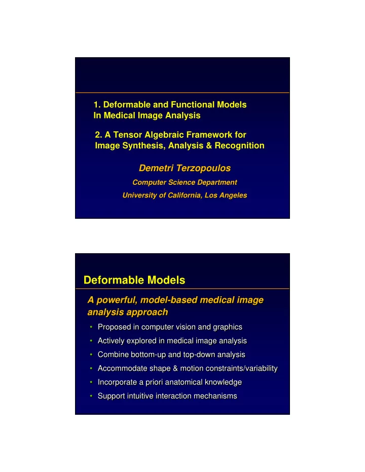
1. Deformable and Functional Models In Medical Image Analysis 2. A Tensor Algebraic Framework for Image Synthesis, Analysis & Recognition Demetri Terzopoulos Terzopoulos Demetri Computer Science Department Computer Science Department University of California, Los Angeles University of California, Los Angeles Deformable Models A powerful, model- A powerful, model -based medical image based medical image A powerful, model-based medical image analysis approach analysis approach analysis approach • • Proposed in computer vision and graphics Proposed in computer vision and graphics • Proposed in computer vision and graphics • Actively explored in medical image analysis Actively explored in medical image analysis • • Actively explored in medical image analysis • Combine bottom Combine bottom- -up and top up and top- -down analysis down analysis • • Combine bottom-up and top-down analysis • Accommodate shape & motion constraints/variability Accommodate shape & motion constraints/variability • • Accommodate shape & motion constraints/variability • • Incorporate a priori anatomical knowledge Incorporate a priori anatomical knowledge • Incorporate a priori anatomical knowledge • Support intuitive interaction mechanisms • Support intuitive interaction mechanisms • Support intuitive interaction mechanisms

Computing Visible Surfaces from Scattered Visual Data [Terzopoulos, 1984] Thin Thin- -plate plate spline spline under tension under tension Thin-plate spline under tension { } { } z x x y y z z c c z ( , ), , data point: ( , ), , 1 ∑ 1 ∑ k k k k k k k k = − E = c z − f x y E c z f x y 2 [ ( , ) ] 2 [ ( , ) ] d k k k k d k k k k z z k 2 2 k k k c c k k f x y f x y ( , ) ( , ) y y x k y x k y ( , ) ( , ) k k x x ρ ( [ ) ( ) ] [ ( ) ( ) ] 1 1 ∫∫ ∫∫ = ρ τ + + − τ + + = τ + + − τ + + E f f 2 f 2 f 2 f 2 f 2 d x d y E f f 2 f 2 f 2 f 2 f 2 d x d y ( ) ( 1 ) 2 ( ) ( 1 ) 2 x y xx xy yy x y xx xy yy 2 2 Discontinuity-Preserving Surface Reconstruction Make Make “ “rigidity rigidity” ” & & “ “tension tension” ” functions of (x,y) functions of (x,y) •Tangent discontinuities: Tangent discontinuities: • τ = τ x y = x y ( , ) 1 ( , ) 1 •Jump discontinuities: Jump discontinuities: • ρ = ρ = x y x y ( , ) 0 ( , ) 0

Snakes: Active Contours [Kass, Witkin, Terzopoulos, 1987] • Curve representation: Curve representation: • • Curve representation: ⎡ ⎤ ⎡ x u t ⎤ x u t ( , ) ( , ) = ∈ = ∈ u t u u t ⎢ ⎥ u c ( , ) ⎢ ⎥ ; [ 0 , 1 ] c ( , ) ; [ 0 , 1 ] y u t ⎣ y u t ⎦ ⎣ ( , ) ⎦ ( , ) 2 2 ∂ 2 ∂ ∂ 2 ∂ 2 2 1 c c 1 c c ∫ 1 ∫ 1 = + E = w + w d u • Curve deformation energy: Curve deformation energy: E w w d u • • Curve deformation energy: ( c ) ( c ) ∂ ∂ 1 ∂ 2 ∂ 1 u 2 u 2 u u 2 2 2 0 0 µ + γ + δ = µ + γ + δ = & & & E & & & E c c ( c ) f • Equations of motion: • Equations of motion: c c ( c ) f • Equations of motion: c c ⎛ ⎞ ∂ ∂ ∂ ⎛ ∂ ⎞ ∂ ⎛ ∂ ⎞ ∂ ∂ ⎛ ⎞ 2 2 2 2 c c c c ⎜ ⎟ µ + γ − + ⎜ ⎟ = µ + γ − ⎜ w ⎟ + w = & & & ⎜ w ⎟ w & & & c c f c c ⎜ ⎟ f ⎜ ⎟ ∂ ∂ ∂ ∂ ∂ 1 ∂ ∂ 2 ∂ u ⎝ 1 u ⎠ u 2 2 u 2 u ⎝ u ⎠ u 2 u 2 ⎝ ⎠ ⎝ ⎠ Image Analysis Using Snakes External forces come from an image External forces come from an image External forces come from an image = −∇ = −∇ P P f ( c ) f ( c ) P x y P x y • Image potential: Image potential: • • Image potential: ( , ) ( , )

Motion Tracking in Video Time Time- -varying image potential varying image potential Time-varying image potential P x y t P x y t ( , , ) ( , , ) Snake-Based Tracking (Blake & (Blake & Isard Isard, Oxford University) , Oxford University) (Blake & Isard, Oxford University)

Discretization • Continuous equations of motion Continuous equations of motion • • Continuous equations of motion ⎛ ⎞ ∂ ∂ ∂ ⎛ ∂ ⎞ ∂ ⎛ ∂ ⎞ ∂ ∂ ⎛ ⎞ 2 2 2 2 c c c c ⎜ ⎟ µ + γ − + ⎜ ⎟ = µ + γ − ⎜ w ⎟ + w = & & & ⎜ w ⎟ w & & & c c f c c ⎜ ⎟ f ⎜ ⎟ ∂ ∂ ∂ ∂ ∂ u ⎝ 1 1 ∂ u ⎠ ∂ u 2 2 ∂ u u ⎝ u ⎠ u 2 u 2 2 ⎝ 2 ⎠ ⎝ ⎠ • Discrete equations of motion • Discrete equations of motion • Discrete equations of motion + + = + + = & & & & & & M c D c Kc f M c D c Kc f Mass matrix Stiffness External forces matrix Damping matrix Snake Stiffness Matrix ⎡ ⎤ ⎡ a b c c b ⎤ a b c c b N − N − 0 0 0 N − 2 N − 1 Finite differences: Finite differences: 0 0 0 2 1 Finite differences: ⎢ ⎥ ⎢ ⎥ b a b c c b a b c c ⎢ ⎥ ⎢ ⎥ − N − 0 1 1 1 N 1 0 1 1 1 1 ⎢ ⎥ = = − ⎢ ⎥ = ih i = N − c b a b c ih i L N c b a b c c c ( ); 0 , L , 1 c c ( ); 0 , , 1 i i 0 1 2 2 2 ⎢ 0 1 2 2 2 ⎥ ⎢ ⎥ c b a b c c b a b c ⎢ ⎥ ⎢ ⎥ = = 1 2 3 3 3 1 2 3 3 3 K K ⎢ ⎥ ⎢ ⎥ ∂ − ∂ − O O O O O O O O O O c c c c c c ≈ + ≈ i + i ⎢ ⎥ i 1 i ⎢ ⎥ 1 ∂ ∂ u h c b a b c u h ⎢ c b a b c ⎥ ⎢ ⎥ − − − − − N − N − N − N − N − N 5 N 4 N 3 N 3 N 3 5 4 3 3 3 ⎢ ⎥ ⎢ ⎥ ∂ − + ∂ 2 − + 2 c c 2 c c c c b a b c c 2 c c c c b a b ≈ ≈ i + i i − ⎢ ⎥ i + 1 i i − 1 ⎢ N − N − N − N − N − ⎥ 1 1 N − 2 N − 4 N − 3 N − 2 N − 2 2 4 3 2 2 ∂ ∂ u h u 2 h 2 2 2 ⎢ b c c b a ⎥ ⎢ b c c b a ⎥ ⎣ ⎣ ⎦ ⎦ − − − − − N − N − N − N − N − N 1 N 1 N 3 N 2 N 1 1 1 3 2 1 + + + w + w w + w + w w w w w w 4 4 − − + = i − i + i − i i + a = 1 ; i 1 1 ; i + 2 ; i 1 2 ; i 2 ; i 1 a 1 ; 1 1 ; 2 ; 1 2 ; 2 ; 1 i i h 2 h 4 h 2 h 4 + w w + w w w w 2 2 2 2 + = − i − i i + b = − 1 ; i − 2 ; i 2 ; i 1 b 1 ; 2 ; 2 ; 1 i = i w = w ih h 2 h 4 w w ih h 2 h 4 ( ) ( ) i 1 ; i 1 1 ; 1 w w = w = w ih w w ( ih ) + ( ) = i + c = 2 ; i 1 c 2 ; 1 i 2 ; i 2 2 ; 2 i i h 4 h 4