Defmod 1 : Finite element code for modeling crustal deformation - - PowerPoint PPT Presentation

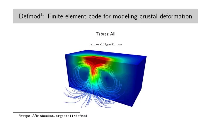
Defmod1: Finite element code for modeling crustal deformation

Tabrez Ali

tabrezali@gmail.com

1https://bitbucket.org/stali/defmod

Features

– Can simulate elastodynamic & quasistatic processes (in 2D or 3D) such as: – Coseismic (fault) slip or volcanic rifting – Postseismic or postrifting deformation due to afterslip, poroelastic rebound and/or viscoelastic relaxation – Postglacial rebound and hydrological (un)loading – Injection/extraction of fluids from subsurface reservoirs etc. – Written entirely in Fortran 95 – Uses PETSc’s parallel sparse data structures & solvers – Runs on shared and distributed memory machines using MPI – Scales well on large clusters with hundreds or even thousands of processor cores – Free to download, use, modify and share (GPL v3)

Features

Supports: – Stabilized linear tri, quad, tet & hex elements – Elastic, viscoelastic, poroelastic and poroviscoelastic rheologies – Time dependent force/flow and/or traction/flux BC’s – Time dependent linear constraint equations – Absorbing boundaries for dynamic problems – Winkler foundation(s) Note(s): – Fault slip/opening and displacement/velocity/pressure BC’s can be specified using linear constraint equations – Isostasy can be simulated using Winkler foundation(s)

Physics

Cauchy’s equation of motion:

• Ω

(σij,j + fi − ρ¨ ui)dΩ = 0 Semi discrete form using the finite element method: M¨ u + C ˙ u + Ku = f C = αM + βK – M is the mass matrix – K is the stiffness matrix – C is the damping matrix – α and β are Rayleigh damping coefficients

Constraint Equations

Implemented using Lagrange Multipliers M¨ u + C ˙ u + Ku + G Tλ = f Gu = l – G is the constraint matrix – λ is the force required to enforce the constraint – l is the value of the constraint (e.g., prescribed slip or displacements)

Explicit Solver for Dynamic problems

For problems without constraints we perform explicit time integration using a central differencing scheme for ¨ u and a backward differencing scheme for ˙ u ut+∆t =M−1 ∆t2(f − Kut) − ∆tC(ut − ut−∆t)

• +

2ut − ut−∆t – M is assumed to be lumped (i.e., diagonal) – Time step is restricted by ∆tcritical ∼ L/c; c =

• E/ρ

where L is the (smallest) element length For problems with constraints we use the “Forward Increment Lagrange Multiplier Method” of Carpenter et al. [1991]

Implicit Solver for Quasistatic problems

– With linear constraints (LM’s)

• K

G T G

• u

λ

• =
• f

l

• System is indefinite and solved using ASM preconditioned GMRES

– Without constraints

• K
• u
• =
• f
• System is symmetric positive definite and CG can be used instead (-ksp type cg)

Note: PETSc can be configured with many sparse solvers and preconditioners that can be engaged at runtime by simple command line options

Implicit Solver for Quasistatic problems

– For problems involving viscoelasticity we use the time-stepping algorithm proposed by Melosh and Raefsky [1980] – For poroelastic problems we also have to account for the continuity equation which results in the coupled system [Zienkiewicz and Shiomi, 1984]: Keu − Hp = f HT ˙ u + S ˙ p + Kcp = q where Ke and Kc are solid and fluid stiffness matrices, H is the coupling matrix, S is the compressibility matrix, p the pressure vector and q the in/out flow The equations are solved using an incremental loading scheme [Smith and Griffiths, 2004]

Implicit Solver for Quasistatic problems

– For problems involving viscoelasticity we use the time-stepping algorithm proposed by Melosh and Raefsky [1980] – For poroelastic problems we also have to account for the continuity equation which results in the coupled system [Zienkiewicz and Shiomi, 1984]: Keu − Hp = f HT ˙ u + S ˙ p + Kcp = q where Ke and Kc are solid and fluid stiffness matrices, H is the coupling matrix, S is the compressibility matrix, p the pressure vector and q the in/out flow The equations are solved using an incremental loading scheme [Smith and Griffiths, 2004]

Applications

Many ...

Applications

Including problems with non-trivial fault geometries Model with ∼ 8 million tet elements, with slip on the entire subduction interface, implicitly solved, from start to finish, in ∼ 120 secs on 256 Xeon E5-2660 cores

Applications

Complex loading histories Model with ∼ 6 million tet elements, with a slipping strike slip fault, explicitly solved (includes 2000 time steps), from start to finish, in ∼ 47.5 secs on 128 cores

Applications

Realistic topography Model (mesh built by T. Masterlark) containing a spherical magma chamber, with traction loading on the chamber wall, implicitly solved, from start to finish, in ∼ 1.5 secs on 4 cores

Applications

Heterogeneous (3D) material properties A full 200 sec simulation of long-period (∼ 0.075 Hz) ground motion in Southern California, using SCEC’s CVM-S4, due to slip on the Southern San Andreas Fault takes ∼ 100 secs on 256 cores

Applications

Fully coupled multiphysics Model containing a porous, permeable magma chamber; Mass flux at the base of the conduit results in ∆P (left) which then causes uplift (right)

I/O

Input – A single ASCII file is used for ease of use and easy manipulation of mesh/BCs for runs driven by shell scripts – Currently all processor cores access the same ASCII input file2 to read on-core (i.e., local) mesh data Output – Each processor core writes its own ASCII output (VTK) for on-core elements/nodes that can be directly visualized using ParaView – Output frequency can be specified in the input file (e.g., write output after every 50 time steps)

2Can take a few minutes for runs involving more than 1K processor cores; E.g., 3 mins to partition, read and

map a ∼16 million (hex) element mesh on 1K cores of Lonestar (TACC) cluster

Input file example

$ cat examples/two quads qs.inp implicit quad 6 2 6 2 0 2 0 0 0.0 0.1 1 1 1 2 3 4 1 2 5 6 3 2 0.00 0.00 0 0 10.0 0.00 1 1 10.0 10.0 1 1 0.00 10.0 0 0 20.0 0.00 1 1 20.0 10.0 1 1 3.0E10 0.25 1.0E18 1.0 3000.0 3.0E10 0.25 1.0E18 1.0 3000.0 5 -10.0E10 0.0 0.0 0.0 6 -10.0E10 0.0 0.0 0.0

Input file example

$ cat examples/two quads qs.inp implicit quad 6 2 6 2 0 2 0 0 0.0 0.1 1 1 1 2 3 4 1 Element data 2 5 6 3 2 0.00 0.00 0 0 10.0 0.00 1 1 10.0 10.0 1 1 0.00 10.0 0 0 20.0 0.00 1 1 20.0 10.0 1 1 3.0E10 0.25 1.0E18 1.0 3000.0 3.0E10 0.25 1.0E18 1.0 3000.0 5 -10.0E10 0.0 0.0 0.0 6 -10.0E10 0.0 0.0 0.0

Input file example

$ cat examples/two quads qs.inp implicit quad 6 2 6 2 0 2 0 0 0.0 0.1 1 1 1 2 3 4 1 2 5 6 3 2 0.00 0.00 0 0 Nodal Data 10.0 0.00 1 1 10.0 10.0 1 1 0.00 10.0 0 0 20.0 0.00 1 1 20.0 10.0 1 1 3.0E10 0.25 1.0E18 1.0 3000.0 3.0E10 0.25 1.0E18 1.0 3000.0 5 -10.0E10 0.0 0.0 0.0 6 -10.0E10 0.0 0.0 0.0

Input file example

$ cat examples/two quads qs.inp implicit quad 6 2 6 2 0 2 0 0 0.0 0.1 1 1 1 2 3 4 1 2 5 6 3 2 0.00 0.00 0 0 10.0 0.00 1 1 10.0 10.0 1 1 0.00 10.0 0 0 20.0 0.00 1 1 20.0 10.0 1 1 3.0E10 0.25 1.0E18 1.0 3000.0 Material data 3.0E10 0.25 1.0E18 1.0 3000.0 5 -10.0E10 0.0 0.0 0.0 6 -10.0E10 0.0 0.0 0.0

Input file example

$ cat examples/two quads qs.inp implicit quad 6 2 6 2 0 2 0 0 0.0 0.1 1 1 1 2 3 4 1 2 5 6 3 2 0.00 0.00 0 0 10.0 0.00 1 1 10.0 10.0 1 1 0.00 10.0 0 0 20.0 0.00 1 1 20.0 10.0 1 1 3.0E10 0.25 1.0E18 1.0 3000.0 3.0E10 0.25 1.0E18 1.0 3000.0 5 -10.0E10 0.0 0.0 0.0 Applied (nodal) force data 6 -10.0E10 0.0 0.0 0.0

Input file example

$ cat examples/two quads qs.inp implicit quad 6 2 6 2 0 2 0 0 0.0 0.1 1 1 1 2 3 4 1 2 5 6 3 2 0.00 0.00 0 0 10.0 0.00 1 1 10.0 10.0 1 1 0.00 10.0 0 0 20.0 0.00 1 1 20.0 10.0 1 1 3.0E10 0.25 1.0E18 1.0 3000.0 3.0E10 0.25 1.0E18 1.0 3000.0 5 -10.0E10 0.0 0.0 0.0 Start and end time(s) for applied force 6 -10.0E10 0.0 0.0 0.0

Input file example

$ cat examples/two quads qs.inp implicit quad 6 2 6 2 0 2 0 0 0.0 0.1 1 1 Total simulation time 1 2 3 4 1 2 5 6 3 2 0.00 0.00 0 0 10.0 0.00 1 1 10.0 10.0 1 1 0.00 10.0 0 0 20.0 0.00 1 1 20.0 10.0 1 1 3.0E10 0.25 1.0E18 1.0 3000.0 3.0E10 0.25 1.0E18 1.0 3000.0 5 -10.0E10 0.0 0.0 0.0 6 -10.0E10 0.0 0.0 0.0

Input file example

$ cat examples/two quads qs.inp implicit quad 6 2 6 2 0 2 0 0 0.0 0.1 1 1 Time step 1 2 3 4 1 2 5 6 3 2 0.00 0.00 0 0 10.0 0.00 1 1 10.0 10.0 1 1 0.00 10.0 0 0 20.0 0.00 1 1 20.0 10.0 1 1 3.0E10 0.25 1.0E18 1.0 3000.0 3.0E10 0.25 1.0E18 1.0 3000.0 5 -10.0E10 0.0 0.0 0.0 6 -10.0E10 0.0 0.0 0.0

Input file example

$ cat examples/two quads qs.inp implicit quad 6 2 6 2 0 2 0 0 0.0 0.1 1 1 Output frequency 1 2 3 4 1 2 5 6 3 2 0.00 0.00 0 0 10.0 0.00 1 1 10.0 10.0 1 1 0.00 10.0 0 0 20.0 0.00 1 1 20.0 10.0 1 1 3.0E10 0.25 1.0E18 1.0 3000.0 3.0E10 0.25 1.0E18 1.0 3000.0 5 -10.0E10 0.0 0.0 0.0 6 -10.0E10 0.0 0.0 0.0

Input file example

$ cat examples/two quads qs.inp implicit quad 6 2 6 2 0 2 0 0 0.0 0.1 1 1 Write total displacements 1 2 3 4 1 2 5 6 3 2 0.00 0.00 0 0 10.0 0.00 1 1 10.0 10.0 1 1 0.00 10.0 0 0 20.0 0.00 1 1 20.0 10.0 1 1 3.0E10 0.25 1.0E18 1.0 3000.0 3.0E10 0.25 1.0E18 1.0 3000.0 5 -10.0E10 0.0 0.0 0.0 6 -10.0E10 0.0 0.0 0.0

Build and Execution

$ ssh lonestar.tacc.utexas.edu $ module load petsc $ git clone https://bitbucket.org/stali/defmod $ cd defmod $ make all $ mpirun -np 2 ./defmod -f examples/two quads qs.inp Reading input file ... Partitioning mesh ... Forming [K] ... Forming RHS ... Setting up solver ... Solving ... Recovering stress ... Cleaning up ... Finished

Build and Execution

$ ssh lonestar.tacc.utexas.edu $ module load petsc $ git clone https://bitbucket.org/stali/defmod $ cd defmod $ make all $ mpirun -np 2 ./defmod -f examples/two quads qs.inp -ksp monitor Reading input file ... Partitioning mesh ... Forming [K] ... Forming RHS ... Setting up solver ... Solving ... 0 KSP Residual norm 6.484684701823e+00 1 KSP Residual norm 2.983375739070e-15 Recovering stress ... Cleaning up ... Finished

Build and Execution

$ ssh lonestar.tacc.utexas.edu $ module load petsc $ git clone https://bitbucket.org/stali/defmod $ cd defmod $ make all $ mpirun -np 2 ./defmod -f examples/two quads qs.inp -ksp monitor Reading input file ... Partitioning mesh ... Forming [K] ... Forming RHS ... Setting up solver ... Solving ... 0 KSP Residual norm 6.484684701823e+00 1 KSP Residual norm 2.983375739070e-15 Recovering stress ... Cleaning up ... Finished By default output is written in VTK format and can be easily visualized using ParaView, VisIt etc.

Result

Input file with constraints

$ cat examples/quadtree qs.inp implicit quad 12 10 19 1 10 0 0 0 1.0 0.25 1 1 1 2 5 4 1 ... 0.0 0.0 0 0 ... 7.5E10 0.25 1.0E18 1.0 3000.0 3 1.0 0.0 5 1.0 0.0 8

• 2.0 0.0 13

0.0 0.0 0.0

• 3

0.0 1.0 5 0.0 1.0 8 0.0 -2.0 13 0.0 0.0 0.0 ... 1 1.0 0.0 9 1.0 0.0 1.0 1 0.0 1.0 9 1.0 0.0 1.0

Input file with constraints

$ cat examples/quadtree qs.inp implicit quad 12 10 19 1 10 0 0 0 Constraint Eqn’s 1.0 0.25 1 1 1 2 5 4 1 ... 0.0 0.0 0 0 ... 7.5E10 0.25 1.0E18 1.0 3000.0 3 1.0 0.0 5 1.0 0.0 8

• 2.0 0.0 13

0.0 0.0 0.0

• 3

0.0 1.0 5 0.0 1.0 8 0.0 -2.0 13 0.0 0.0 0.0 ... 1 1.0 0.0 9 1.0 0.0 1.0 1 0.0 1.0 9 1.0 0.0 1.0

Input file with constraints

$ cat examples/quadtree qs.inp implicit quad 12 10 19 1 10 0 0 0 1.0 0.25 1 1 1 2 5 4 1 ... 0.0 0.0 0 0 ... 7.5E10 0.25 1.0E18 1.0 3000.0 3 Equation 1 {Ux5+Ux8-2Ux13=0.0} 1.0 0.0 5 1.0 0.0 8

• 2.0 0.0 13

0.0 0.0 0.0

• 3

0.0 1.0 5 0.0 1.0 8 0.0 -2.0 13 0.0 0.0 0.0 ... 1 1.0 0.0 9 1.0 0.0 1.0 1 0.0 1.0 9 1.0 0.0 1.0

Input file with constraints

$ cat examples/quadtree qs.inp implicit quad 12 10 19 1 10 0 0 0 1.0 0.25 1 1 1 2 5 4 1 ... 0.0 0.0 0 0 ... 7.5E10 0.25 1.0E18 1.0 3000.0 3 1.0 0.0 5 1.0 0.0 8

• 2.0 0.0 13

0.0 0.0 0.0 Start and end time(s)

• 3

0.0 1.0 5 0.0 1.0 8 0.0 -2.0 13 0.0 0.0 0.0 ... 1 1.0 0.0 9 1.0 0.0 1.0 1 0.0 1.0 9 1.0 0.0 1.0

Input file with constraints

$ cat examples/quadtree qs.inp implicit quad 12 10 19 1 10 0 0 0 1.0 0.25 1 1 1 2 5 4 1 ... 0.0 0.0 0 0 ... 7.5E10 0.25 1.0E18 1.0 3000.0 3 1.0 0.0 5 1.0 0.0 8

• 2.0 0.0 13

0.0 0.0 0.0

• 3 Equation 2 {Uy5+Uy8-2Uy13=0.0}

0.0 1.0 5 0.0 1.0 8 0.0 -2.0 13 0.0 0.0 0.0 ... 1 1.0 0.0 9 1.0 0.0 1.0 1 0.0 1.0 9 1.0 0.0 1.0

Input file with constraints

$ cat examples/quadtree qs.inp implicit quad 12 10 19 1 10 0 0 0 1.0 0.25 1 1 1 2 5 4 1 ... 0.0 0.0 0 0 ... 7.5E10 0.25 1.0E18 1.0 3000.0 3 1.0 0.0 5 1.0 0.0 8

• 2.0 0.0 13

0.0 0.0 0.0

• 3

0.0 1.0 5 0.0 1.0 8 0.0 -2.0 13 0.0 0.0 0.0 ... 1 Equation 9 {Ux9=1.0} 1.0 0.0 9 1.0 0.0 1.0 1 0.0 1.0 9 1.0 0.0 1.0

Input file with constraints

$ cat examples/quadtree qs.inp implicit quad 12 10 19 1 10 0 0 0 1.0 0.25 1 1 1 2 5 4 1 ... 0.0 0.0 0 0 ... 7.5E10 0.25 1.0E18 1.0 3000.0 3 1.0 0.0 5 1.0 0.0 8

• 2.0 0.0 13

0.0 0.0 0.0

• 3

0.0 1.0 5 0.0 1.0 8 0.0 -2.0 13 0.0 0.0 0.0 ... 1 1.0 0.0 9 1.0 0.0 1.0 1 Equation 10 {Uy9=1.0} 0.0 1.0 9 1.0 0.0 1.0

Input file with constraints

$ cat examples/quadtree qs.inp implicit quad 12 10 19 1 10 0 0 0 1.0 0.25 1 1 1 2 5 4 1 ... 0.0 0.0 0 0 ... 7.5E10 0.25 1.0E18 1.0 3000.0 3 1.0 0.0 5 1.0 0.0 8

• 2.0 0.0 13

0.0 0.0 0.0

• 3

0.0 1.0 5 0.0 1.0 8 0.0 -2.0 13 0.0 0.0 0.0 ... 1 1.0 0.0 9 1.0 0.0 1.0 1 0.0 1.0 9 1.0 0.0 1.0

Note: Any constraint that is specified remains active throughout the simulation; A zero value is assumed (for u or p) unless specified otherwise

Result

Note: Displacements at hanging nodes are average of their corresponding edge nodes

More examples ...

– Displacement BC in 3D Uy9=10.0

1 0.0 1.0 0.0 9 10.0 0.0 0.0 – Pressure head BC in 3D (for poroelastic problem) P9=1.0E3 1 0.0 0.0 0.0 1.0 9 1.0E3 0.0 0.0 – Fault slip between two coincident nodes (in x-direction) Ux13-Ux81=10.0 2 1.0 0.0 0.0 13

• 1.0 0.0 0.0 81

10.0 0.0 0.0

More examples ...

– Displacement BC in 3D Uy9=10.0

1 0.0 1.0 0.0 9 10.0 0.0 0.0 – Pressure head BC in 3D (for poroelastic problem) P9=1.0E3 1 0.0 0.0 0.0 1.0 9 1.0E3 0.0 0.0 – Fault slip between two coincident nodes (in x-direction) Ux13-Ux81=10.0 2 1.0 0.0 0.0 13

• 1.0 0.0 0.0 81

10.0 0.0 0.0

More examples ...

– Displacement BC in 3D Uy9=10.0

1 0.0 1.0 0.0 9 10.0 0.0 0.0 – Pressure head BC in 3D (for poroelastic problem) P9=1.0E3 1 0.0 0.0 0.0 1.0 9 1.0E3 0.0 0.0 – Fault slip between two coincident nodes (in x-direction) Ux13-Ux81=10.0 2 1.0 0.0 0.0 13

• 1.0 0.0 0.0 81

10.0 0.0 0.0

Fault slip

El−1 El−2 4 1 3 2 5 Element view Nodal view (exploded) 6 7 8

To enforce slip we need to specify the relative displacement/opening between coincident nodes {3 & 8} and {2 & 5} For example the relative displacement (Y coordinate) between nodes {3 & 8} can be written as Uy3-Uy8=1.0 and is specified (between 0.1 − 0.5 seconds) as:

2 1 3 0 -1 8 1.0 0.1 0.5

Fault slip

Example

$ cat examples/2d fault dyn.inp explicit quad 12 18796 19036 2 48 0 0 200 75 0.025 40 0 0.0 0.01 ... 2 0 -1 1832 1 1619 0.1 0.2 2.7 2 1 0 1832

• 1 0 1619

0.1 0.2 2.7 ...

Example

$ cat examples/2d fault dyn.inp explicit quad 12 18796 19036 2 48 0 0 200 ABC’s 75 0.025 40 0 0.0 0.01 ... 2 0 -1 1832 1 1619 0.1 0.2 2.7 2 1 0 1832

• 1 0 1619

0.1 0.2 2.7 ...

Example

$ cat examples/2d fault dyn.inp explicit quad 12 18796 19036 2 48 0 0 200 75 0.025 40 0 0.0 0.01 Damping coefficients ... 2 0 -1 1832 1 1619 0.1 0.2 2.7 2 1 0 1832

• 1 0 1619

0.1 0.2 2.7 ...

Example (Dynamic)

T=0.0 sec Displacement Velocity (100x)

Example (Dynamic)

T=2.5 sec Displacement Velocity (100x)

Example (Dynamic)

T=5.0 sec Displacement Velocity (100x)

Example (Dynamic)

T=7.5 sec Displacement Velocity (100x)

Example (Dynamic)

T=10.0 sec Displacement Velocity (100x)

Example (Dynamic)

T=12.5 sec Displacement Velocity (100x)

Example (Dynamic)

T=15.0 sec Displacement Velocity (100x)

Example (Dynamic)

T=17.5 sec Displacement Velocity (100x)

Example (Dynamic)

T=20.0 sec Displacement Velocity (100x)

Example (Dynamic)

T=22.5 sec Displacement Velocity (100x)

Example (Dynamic)

T=25.0 sec Displacement Velocity (100x)

Example (Dynamic)

T=27.5 sec Displacement Velocity (100x)

Example (Dynamic)

T=30.0 sec Displacement Velocity (100x)

Example (Dynamic)

T=32.5 sec Displacement Velocity (100x)

Example (Quasistatic)

T=0.0 years Displacement Velocity (20x)

Example (Quasistatic)

T=5.0 years Displacement Velocity (20x)

Example (Quasistatic)

T=10.0 years Displacement Velocity (20x)

Example (Quasistatic)

T=15.0 years Displacement Velocity (20x)

Example (Quasistatic)

T=20.0 years Displacement Velocity (20x)

Example (3D Quasistatic)

T=0.0 years (Rifting starts) Displacement

Example (3D Quasistatic)

T=1.0 years (Rifting ...) Displacement

Example (3D Quasistatic)

T=2.0 years (Rifting ...) Displacement

Example (3D Quasistatic)

T=3.0 years (Rifting ...) Displacement

Example (3D Quasistatic)

T=4.0 years (Rifting ...) Displacement

Example (3D Quasistatic)

T=5.0 years (Rifting ends) Displacement

Example (3D Quasistatic)

T=10.0 years (Postrifting viscous relaxation) Displacement

Example (2D Dynamic with ABCs)

Time step 250 Note: Full computational domain is shown

Example (2D Dynamic with ABCs)

Time step 500 Note: Full computational domain is shown

Example (2D Dynamic with ABCs)

Time step 750 Note: Full computational domain is shown

Example (2D Dynamic with ABCs)

Time step 1000 Note: Full computational domain is shown

Example (3D Dynamic)

T=3.0 secs Velocity

Example (3D with Traction BCs)

Deformation due to lake3 loading

3Shoreline is shown in white

Example (2D Poroelasticity)

Pore pressure change following an earthquake at time step 0 (i) with a permeable fault zone (ii) with an impermeable fault zone

Example (2D Poroelasticity)

Pore pressure change following an earthquake at time step 5 (i) with a permeable fault zone (ii) with an impermeable fault zone

Example (2D Poroelasticity)

Pore pressure change following an earthquake at time step 10 (i) with a permeable fault zone (ii) with an impermeable fault zone

Example (2D Poroelasticity)

Pore pressure change following an earthquake at time step 15 (i) with a permeable fault zone (ii) with an impermeable fault zone

Example (2D Poroelasticity)

Pore pressure change following an earthquake at time step 20 (i) with a permeable fault zone (ii) with an impermeable fault zone

Example (2D Poroelasticity)

Pore pressure change due to injection (top right) and withdrawl (top left) of fluid in a saturated reservoir Production on

Example (2D Poroelasticity)

Pore pressure change due to injection (top right) and withdrawl (top left) of fluid in a saturated reservoir Production on

Example (2D Poroelasticity)

Pore pressure change due to injection (top right) and withdrawl (top left) of fluid in a saturated reservoir Production on

Example (2D Poroelasticity)

Pore pressure change due to injection (top right) and withdrawl (top left) of fluid in a saturated reservoir Production on

Example (2D Poroelasticity)

Pore pressure change due to injection (top right) and withdrawl (top left) of fluid in a saturated reservoir Production on

Example (2D Poroelasticity)

Pore pressure change due to injection (top right) and withdrawl (top left) of fluid in a saturated reservoir Production on

Example (2D Poroelasticity)

Pore pressure change due to injection (top right) and withdrawl (top left) of fluid in a saturated reservoir Production on

Example (2D Poroelasticity)

Pore pressure change due to injection (top right) and withdrawl (top left) of fluid in a saturated reservoir Production on

Example (2D Poroelasticity)

Pore pressure change due to injection (top right) and withdrawl (top left) of fluid in a saturated reservoir Production off

Example (2D Poroelasticity)

Pore pressure change due to injection (top right) and withdrawl (top left) of fluid in a saturated reservoir Production off

Example (2D Poroelasticity)

Pore pressure change due to injection (top right) and withdrawl (top left) of fluid in a saturated reservoir Production off

Example (2D Poroelasticity)

Pore pressure change due to injection (top right) and withdrawl (top left) of fluid in a saturated reservoir Production off

Example (2D Poroelasticity)

Fluid velocity vectors (unscaled) during steady production With flow BC

Example (2D Poroelasticity)

Fluid velocity vectors (unscaled) during steady production With no-flow BC

Example (3D Poroelasticity)

Pore pressure change due to withdrawl of fluid from a confined reservoir; Permeability ratio b/w reservoir and surrounding rock = 1.0E6 Note: In 3D, both (stabilized) linear tet or hex elements can be used

Example (3D Poroelasticity)

Pore pressure change due to withdrawl of fluid from a confined reservoir; Permeability ratio b/w reservoir and surrounding rock = 1.0E6 Note: In 3D, both (stabilized) linear tet or hex elements can be used

Parallelism

Each processor core owns only a part of the mesh, part of the stiffness matrix, part of the load/solution vector and writes its own VTK output A mesh partitioned (using METIS) to run on 4 processor cores

Parallelism

Each processor core owns only a part of the mesh, part of the stiffness matrix, part of the load/solution vector and writes its own VTK output Visualization of subdomain(s) 1

Parallelism

Each processor core owns only a part of the mesh, part of the stiffness matrix, part of the load/solution vector and writes its own VTK output Visualization of subdomain(s) 1, 2

Parallelism

Each processor core owns only a part of the mesh, part of the stiffness matrix, part of the load/solution vector and writes its own VTK output Visualization of subdomain(s) 1, 2, 3

Parallelism

Each processor core owns only a part of the mesh, part of the stiffness matrix, part of the load/solution vector and writes its own VTK output Visualization of subdomain(s) 1, 2, 3 and 4

Parallelism

The resulting stiffness matrix, distributed (row wise) across 4 processor cores

Limitations

– Due to the use of a serial mesh partitioner (METIS), the largest problem Defmod can solve on most current generation clusters (having 16−128 GB of RAM on node 0) is limited to 125-1000 million unknowns – Beyond 4000 cores, the ‘I’ part in ‘I/O’ is likely to become a bottleneck as all cores will have to access the same input file to read part of the mesh they own (skipping rest) during the initialization phase

Solver performance

On the Trestles cluster (SDSC) for a problem with ∼ 25 million unknowns ...

CPU Cores DOF per Explicit Dynamic Implicit Quasistatic Used # core Solver Efficiency Solver Efficiency4 128 195.2K 1.00 1.00 256 97.6K 0.97 0.92 512 48.4K 0.93 0.89 1024 24.4K 0.80 0.87 – On most current generation clusters, parallel efficiency of ∼ 90% or more can be achieved as long as DOF/core is > 37.5K – Ideally DOF/core should be b/w 37.5-250K for explicit dynamic problems and b/w 37.5-125K for implicit quasistatic problems (assuming 1GB RAM/core, unbalanced mesh and default solver settings)

4Maximum iterations were fixed

Examples

– Sample files are provided in the examples directory – For more details look at the following files5 in order:

• 1. two quads qs.inp
• 2. quadtree qs.inp
• 3. cube qs.inp
• 4. 2d point load dyn.inp
• 5. 2d fault dyn.inp
• 6. 2d per fault poro qs.inp
• 7. 3d rift visco qs.inp
• 8. 3d traction load qs.inp
• 9. 3d reservoir poro qs.inp

5Some of the files are commented

Showcase application(s)

Investigating source processes; Estimating slip distribution and/or poroviscoelastic properties of rock using (high rate) GPS + InSAR Elastodynamic deformation due to a slipping thrust fault Quasistatic deformation due to afterslip and poroviscoelastic relaxation

TODO

In order of priority

• 1. Code optimization (soon)

– Use adaptive time-stepping for quasistatic problem(s) – Use AMG as default preconditioner for quasistatic problem(s) – Reduce (local) memory footprint by using exact preallocation

• 2. Solution of the adjoint problem (planned)

Source files

Name Description petsc∗.h Header file(s) m utils.F90 Simple utilities (area of triangle/quadrilateral etc.) m elems.F90 Element definitions, shape functions, their derivatives etc. m local.F90 Element level routines to compute stiffness/mass matrix, stress tensor etc. m global.F90 Routines that need access to on-rank arrays (nodal coor- dinates, element connectivity etc.) main.F90 Main code (partitioner/mapper, solver(s) etc.)

More on installation ...

Dependencies

Defmod PETSc METIS MPI BLAS LAPACK

Laptop/PC running Debian

$ sudo apt-get install gcc gfortran make python cmake git $ curl -O http://ftp.mcs.anl.gov/pub/petsc/release-snapshots/petsc-lite-3.12.tar.gz $ tar -xzf petsc-lite-3.12.tar.gz $ cd petsc-3.12.* $ export PETSC DIR=$PWD PETSC ARCH=arch-linux2-c-opt $ ./configure --with-cc=gcc --with-fc=gfortran --download-mpich

• -download-fblaslapack --download-metis --with-debugging=0

$ make all $ export PATH=$PATH:$PETSC DIR/$PETSC ARCH/bin $ git clone https://bitbucket.org/stali/defmod $ cd defmod $ make all $ mpiexec -n 2 ./defmod -f examples/two quads qs.inp -ksp monitor Note: Above instructions can be used on any computer that runs Debian (or Ubuntu); See http://www.debian.org/ports/ for supported architectures

Laptop/PC running Debian

Alternatively, all underlying dependencies (including PETSc and METIS) can be downloaded from the repository. For example:

$ sudo apt-get install libpetsc-real-dev libmetis-dev make git $ git clone https://bitbucket.org/stali/defmod $ cd defmod $ make all PETSC DIR=/usr/lib/petsc FPPFLAGS=-DPETSC HAVE METIS LDLIBS=-lmetis $ mpiexec -n 2 ./defmod -f examples/two quads qs.inp -ksp monitor

Linux clusters

On typical Linux clusters, MPI and BLAS/LAPACK are almost always preinstalled, and all we have to do is:

$ curl -O http://ftp.mcs.anl.gov/pub/petsc/release-snapshots/petsc-lite-3.12.tar.gz $ tar -xzf petsc-lite-3.12.tar.gz $ cd petsc-3.12.* $ export PETSC DIR=$PWD $ ./configure --with-mpi-dir=/path/to/mpi --download-metis --with-debugging=0 $ make all NOTE: /path/to/mpi above is simply the MPI installation directory, which can be be found using: $ which mpif90 | rev | cut -c12- | rev $ git clone https://bitbucket.org/stali/defmod $ cd defmod $ make all $ mpiexec -n 2 ./defmod -f examples/two quads qs.inp -ksp monitor

Linux clusters

On many Linux clusters, such as those available via XSEDE or at large supercomputing centers, PETSc is usually preinstalled. E.g., on the Lonestar cluster at TACC (UTexas) all we have to do is:

$ ssh lonestar.tacc.utexas.edu $ module load petsc $ git clone https://bitbucket.org/stali/defmod $ cd defmod $ make all $ ibrun6 -n 2 -o 0 ./defmod -f examples/two quads qs.inp -ksp monitor

6via Scheduler

Linux clusters

Similarly, on the Comet cluster at SDSC all we have to do is:

$ ssh comet.sdsc.edu $ module load petsc $ git clone https://bitbucket.org/stali/defmod $ cd defmod $ make all PETSC DIR=$PETSCHOME $ ibrun7 ./defmod -f examples/two quads qs.inp -ksp monitor

7via Scheduler

Other Linux distributions and operating systems

– Those using non-Debian based distributions should see the INSTALL file included with the source – Any standard conforming C/Fortran 95 compiler will work. The ones that have been tested and are known to work include: – AOCC (free) – Clang/Flang (free) – Cray – GCC (free) – Intel – Open64 (free) – PGI (free) – Oracle/Sun Studio (free) – Apple macOS and MS Windows users can install all required dependencies using Homebrew and Cygwin/WSL, respectively

Suggested workflow

Cubit or Trelis Exodus II file exo2inp Defmod Input file ParaView VTK output file(s)

Note: The exo2inp utility is available at https://bitbucket.org/stali/defmod-utils/

Derivative work

• Dr. Chunfang Meng at MIT has developed a sophisticated hybrid solver which can simulate

dynamic rupture due to quasistatic loading in poroviscoelastic media, and is useful for studying processes such as induced or triggered seismicity. See https://doi.org/10.1016/j.cageo.2016.11.014 for details. He has combined the hybrid solver with OpenSWPC, a parallel, higher-order finite difference code developed by Takuto Maeda at ERI (University of Tokyo). For more information about this mixed (FE-FD) approach, see https://doi.org/10.1016/j.cageo.2018.01.015.

• Dr. Meng has also extended the code to incorporate fault zone inhomogeneities (damage) as

well as the ability to model slip/rupture on truly intersecting faults. For details, see https://doi.org/10.1785/0220190083 and https://doi.org/10.1785/0220190234, respectively. Defmod has also been incorporated into Esh3D for solving Eshelby’s inclusion problem in full and half space. See https://doi.org/10.1029/2018EA000442 for details.

Acknowledgements

– PETSc team for providing a first class Fortran API and support – Greg Lyzenga/Jay Parker (JPL) for providing the 3D viscoelastic strain rate matrices – Chris Kyriakopoulos (UC Riverside) for his help in validating Defmod with ABAQUS – XSEDE award for testing and benchmarking code on x86 Linux clusters For more information visit https://bitbucket.org/stali/defmod A short preprint describing Defmod is available at http://arxiv.org/abs/1402.0429 Some useful utilities/scripts are available at https://bitbucket.org/stali/defmod-utils