Deep Restricted Bayesian Network BESOM NICE 2017 ... ... ... - PowerPoint PPT Presentation

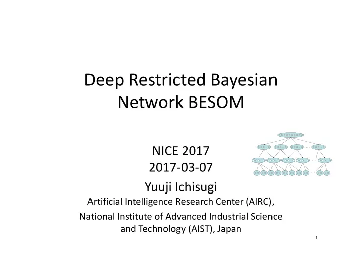
Deep Restricted Bayesian Network BESOM NICE 2017 ... ... ... 。。。 ... ... ... ... ... 。。。 ... 2017-03-07 。。。 Yuuji Ichisugi Artificial Intelligence Research Center (AIRC), National Institute of Advanced Industrial Science and Technology (AIST), Japan 1

BESOM (BidirEctional Self Organizing Maps) [Ichisug 2007] • A computational model of the cerebral cortex – A model of column network , not spiking neurons • Design goals: – Scalability of computation – Usefulness as a machine learning system – Plausibility as a neuroscientific model • As a long-term goal, we aim to reproduce functions of such as the visual areas and the language areas using this cerebral cortex model. 2

Architecture of BESOM model Recognition step: The entire network behaves like a Bayesian network . Learning step: Each node behaves like a Self-organizing map . Node = random variable = macro-column Unit = value of random variable = minicolumn (V2) (V1) (LGN)

Outline • Bayesian networks and the cerebral cortex • BESOM Ver.3 and robust pattern recognition • Toward BESOM Ver.4

Models of visual cortex based on Bayesian networks • Various functions, illusions, neural responses and anatomical structure of the visual cortex were reproduced by Bayesian network models. – [Tai Sing Lee and Mumford 2003] – [George and Hawkins 2005] – [Rao 2005] – [Ichisugi 2007] – [Litvak and Ullman 2009] – [Chikkerur, Serre, Tan and Poggio 2010] – [Hosoya 2012] – ... The visual cortex seems to be a huge Bayesian network with layered structure like Deep Neural Networks.

What is Bayesian networks? – Efficient and expressive data structure of probabilistic knowledge [Perl 1988] • Various probabilistic inference can be executed efficiently if a joint probability table can be factored into small conditional probability tables (CPTs) .  P ( S , W , R , C ) P ( W | S , R ) P ( C | R ) P ( S ) P ( R ) CPTs P(S=yes) P(R=yes) 0.2 0.02 S R S R P(W=yes|S,R) R P(C=yes|R) no no 0.12 no 0.3 no yes 0.8 yes 0.995 W C yes no 0.9 yes yes 0.98 6

Loopy Belief Propagation [Weiss and Freedman 2001] • Efficient approximate inference algorithm – Iterative algorithm with local and asynchronous computation , like brain. – Although there is no guarantee of convergence, it is empirically accurate. ...    BEL ( x ) ( x ) ( x ) U1 Um      ( x ) P ( x | u , , u ) ( u )  1 m X k π X (u k ) λ X (u k ) u ,  , u k 1 m     ( x ) ( x ) X Y l l      π Yl (x) λ Yl (x) ( x ) ( x ) ( x ) Y Y l j  j l        ( u ) ( x ) P ( x | u , , u ) ( u ) ...  Y1 Yn X k 1 m X i  x u , , u / u i k  1 m k 7

Belief propagation and micro circuit of cerebral cortex • The similarity between belief propagation and the six-layer structure of the cerebral cortex has been pointed out many times. [George and Hawkins 2005] [Ichisugi 2007] I [Rohrbein, Eggert and Korner 2008] II [Litvak and Ullman 2009] III IV V VI 8

Approximate Belief Propagation    t 1 t t [Ichisugi 2007] l z W o XY Y XY Y   Approximates Pearl's algorithm [Pearl 1988]    t 1 t 1 o l with some assumptions. X XY  Y children ( X ) � � � � ���   t 1 T t k W b UX UX U     U t 1 t 1 p k X UX b W  U parents ( X ) U UX Z , o X X      t 1 t 1 t 1 r o p X X X X b  W X          t 1 t 1 t 1 t 1 t 1 Z ( r ) ( r o p ) XY Z , ο X X i X X X Y Y 1 Y i      t 1 t 1 t 1 t 1 T z ( Z , Z , , Z )  X X X X     t 1 t 1 t 1 b ( 1 / Z ) r X X X Yuuji ICHISUGI, "The cerebral cortex model that self-organizes   conditional probability tables and executes belief propagation", In T where x y ( x y , x y , , x y )  proc. of IJCNN2007, Aug 2007. 1 1 2 2 n n

Similarity in information flow I [Gilbert 1983] II [Pandya and Yeterian 1985] III IV V Gilbert, C.D., Microcircuitry of the visual-cortex, Annual review of neuroscience, 6: 217-247, 1983. VI Pandya, D.N. and Yeterian, E.H., Architecture and connections of cortical Lower Area Higher Area association areas. In: Peters A, Jones EG, eds. Cerebral Cortex (Vol. 4): Anatomical structure Association and Auditory Cortices. New York: Plenum Press, 3-61, 1985.    t 1 t t l z W o XY Y XY Y      t 1 t 1 o l X XY k k  UX Y children ( X ) XY o o   t 1 T t k W b X Y UX UX U l l  UX XY   t 1  t 1 p k b Z Z X UX b U X Y X  U parents ( X )    t 1  t 1  t 1 r o p X X X Child nodes Parent nodes  t  1  t  1  t  1  t  1  t  1 Z ( r ) ( r o p ) Information flow of the approx. BP X X i X X X 1 i      t 1 t 1 t 1 t 1 T z ( Z , Z , , Z )  X X X X The intermediate variables of this algorithm can be assigned     t 1 t 1 t 1 b ( 1 / Z ) r to each layer of the cerebral cortex without contradicting the X X X known anatomical structure.   T where x y ( x y , x y , , x y )  1 1 2 2 n n

Detailed circuit that calculates the approximate BP ( b ) U 1 1 ( b ) U 2 1 ( b ) U 3 2 ( b ) + + U 1 2 U U ( b ) ( k ) ( k ) U 2 + + 2 U 1 X 1 U 1 X 2 1 2 ( b ) U 3 ( k ) ( k ) 2 U 2 X 1 U 2 X 2 + + ( p ) ( p ) X 1 X 2 X ( o ) ( o ) ( X r ) ( X r ) X 1 X 2 1 2 Z ( l ) ( l ) Y XY 1 XY 2 1 1 1 ( o ) + + Y 1 1 ( o ) Y Y Y 2 1 ( o ) 1 2 Y 3 1 ( l ) ( l ) + + XY 1 XY 2 Z 2 2 Y 2 The left circuit ( o ) Y 1 2 calculates values of ( o ) Y 2 2 two units, x1 and x2, / / ( o ) Y 3 in node X in the above 2 ( b ) ( b ) X 1 X 2 Z network. X + Z X ( o ) ( b ) X 1 X 1 ( o ) ( b ) X 2 X 2

Correspondence with local cortical circuit Mini-column like ( b ) U 1 1 structure ( b ) I U 2 1 ( b ) U 3 2 ( b ) + + U 1 2 ( b ) ( k ) ( k ) II U 2 + + 2 U 1 X 1 U 1 X 2 ( b ) Many horizontal U 3 ( k ) ( k ) 2 U 2 X 1 U 2 X 2 + + fibers in I, IV ( p ) ( p ) X 1 X 2 III ( o ) ( o ) ( X r ) ( X r ) X 1 X 2 1 2 I Z ( l ) ( l ) II Y XY 1 XY 2 1 1 1 ( o ) + + Y 1 III 1 ( o ) Y 2 1 IV ( o ) Y 3 1 ( l ) ( l ) V + + XY 1 XY 2 Z 2 2 IV Y 2 VI ( o ) Y 1 2 ( o ) Y 2 2 / / ( o ) V Y 3 2 Many cells ( b ) ( b ) X 1 X 2 Z VI X in II, IV + Z X ( o ) ( b ) X 1 X 1 ( o ) ( b ) X 2 X 2

Outline • Bayesian networks and the cerebral cortex • BESOM Ver.3 and robust pattern recognition • Toward BESOM Ver.4

Toward realization of the brain function • If the cerebral cortex is a kind of Bayesian network, we should be able to reproduce function and performance of it using Bayesian networks. – As a first step, we aim to reproduce some part of the functions of the visual areas and the language areas. – Although there were some difficulties such as computational cost and local minimum problem, now they have been solved considerably.

BESOM Ver.3.0 features • Restricted Conditional Probability Tables: • Scalable recognition algorithm OOBP [Ichisugi, Takahashi 2015] • Regularization methods to avoid local minima – Win-rate and Lateral-inhibition penalty [Ichisugi, Sano 2016] – Neighborhood learning Yuuji Ichisugi and Naoto Takahashi, Computational amount of An Efficient Recognition Algorithm for Restricted Bayesian Networks, In proc. of IJCNN 2015. one step of iteration of OOBP is linear to the Yuuji Ichisugi and Takashi Sano, Regularization Methods for the Restricted Bayesian number of edges of the Network BESOM, In Proc. of ICONIP2016, Part I, LNCS network. 9947, pp.290--299, 2016. Recognition algorithm OOBP 15

The design of BESOM is motivated by two neuroscientific facts. １．Each macro-column seems to be like a SOM. ２．A macro-column at a upper area receives the output of the macro- columns at the lower area. mini V4 columns ... macro-columns V2 ... ... V1 16

If a SOM receives input from other SOMs, they naturally become a Bayesian Network Learning rule (without neighborhood learning) x     w w ( y w ) i ij ij j ij converges to the probability that fires when fires, that is, the conditional probability w . ij y=(0, 0, 1, 0, 0, 0, 1, 0, 0, 0, 0, 0, 0, 0, 1) T y j 17

Input Node = random variable = macro-column unit = value (V2) = mini- column (V1) (LGN) Input (observed data) is given Connection weights at the lowest layer. = Conditional probabilities = synapse weights Recognition Learning increased decreased Updates connection weights Find the values with the highest posterior with Hebb's rule. probability. (MAP) 18